
Film ROI Project - Web Scraping and Linear Regression
For this project I’m actually revisiting this particular topic. The original version of this project was done at a feverish pace due to time constraints, so I wanted to come back and use the experience as an opportunity to tidy up my approach and learn a new web scraping framework, Scrapy. Some aspects of the tools and methodology might seem like using a bazooka to swat a fly, but on that day when you need a bazooka, you wanted it pointed at the advancing zombie hordes and not your face!
Specifically, this project is an examination of what factors are most important for a film recouping its production budget. Genre, budget, critical reviews, user reviews, opening weekend performance? That last one is of particular interest since there is so much reporting on the subject of opening weekend revenue in film journalism. Generally speaking Hollywood believes that the opening weekend metric is the biggest indicator of overall performance and thus the financial fate of a film. I wanted to see if this was true and or if other factors matter just as much.
To do this I constructed a linear regression model with film data web scraped from IMDb and IMDb Pro. The model will attempt to generate the best prediction possible for the proportion of budget that is recouped at the end of a theatrical run. But the main focus is, given the best model we can produce, which variables contribute most to recouping budget.
Visit the Github repo to see the data, code and notebooks used in the project.
Methodology
- Use the web scraping framework Scrapy, along with Selenium, to gather data on films released 2010 - 2018. This interval was chosen to keep the movies relatively recent and also to ensure that the we had their final box office revenue numbers. Theatrical runs generally only last a few months at the very longest.
- The data gathered is comprised of box office revenue, runtime, critic and user reviews, and genres. This is a mix of pre-release and post release data, which is of dubious value if the only point is to predict performance a significant amount of time before release. However, again the idea is to identify the factors that contribute most strongly to positive budget recoup. I strongly believe that post-release factors can be important to a film’s financial fate (reviews) and are things that filmmakers can adjust and optimize for in the development and production phases of a film.
- Use multiple linear regression models to predict performance and gauge importance of features for the strongest model, employing standard Ordinary Least Squares regression, cross-validation and Ridge and LASSO regularization.
Data
- TARGET - the proportion of budget recouped at the end of a film’s theatrical run (IMDb Pro)
- Genres - genres (up to 3) that the film falls into
- Budget - film production budget (IMDb Pro)
- Opening Revenue - box office revenue for the film’s opening weekend (IMDb Pro)
- North American Revenue - box office revenue for North America (USA + Canada) at the end of a film’s theatrical run (IMDb Pro)
- Total Revenue - worldwide revenue at the end of a film’s theatrical run (IMDb Pro)
- User Rating - IMDb user review rating average (IMDb Pro)
- User Votes - number of user review ratings on IMDb (IMDb Pro)
- Articles - number of articles written about the (IMDb Pro)
- Metacritic - Metacritic aggregate critic rating (IMDb)
- Runtime (IMDb)
Tools
- Python
- Jupyter Notebooks
- Scrapy
- Selenium
- Pandas
- Numpy
- Scikit-learn
- StatsModels
Scrapy + Selenium
In my first stab at this type of project I ended up using Selenium for just about everything. This worked out fine since I was able to get all the data I needed through web page XPaths. However, I had to write a rather monstrous script to do it. On top of that I wrote most of that script in a single cell in a Jupyter notebook which is… suboptimal. Jupyter notebooks are great for tinkering and explorations, but they can fall apart if you try to do any serious scripting. Tough to write them there and they’re, tough to debug. It becomes a frightful mess:
This time around I wanted to both push all of the web scraping into dedicated scripts and to get away with reliance solely on Selenium, which is great for page interactions, but not ideal by itself for complex scraping. I had dabbled with Scrapy before but the learning curve ran head first into my project schedule, but now that I had more time I wanted to dive in and see what I could learn. In the end I used a combination of Selenium and Scrapy, with Scrapy doing most of the work.
Scrape URLs
The first job was to generate the list of films I was going to be working with and get their URLs so I can go to each page and get the data I’m after. This is the place where I definitely needed Selenium. IMDb Pro has an advanced search function that allows you to filter films by various criteria (release date, year, budget, revenue, etc), but you need to click on check boxes and enter text into fields to get this to work. This is theoretically possible with Scrapy, but is MUCH easier in Selenium. However, Scrapy is much better at the mechanics of going from page to page and grabbing data with its spiders, so to keep everything within Scrapy’s framework I put the Selenium code within the Scrapy spider. Here’s a snippet of that code:
class ImdbproSpider(Spider):
    name = 'imdbpro_film_list'
    allowed_domains = ['pro.imdb.com'] # Note here the 'domain' is not like the URL below. No 'https://'
    start_urls = ['https://pro.imdb.com/']

    def parse(self, response):
...
        # Open IMDbPro Log in page
        self.driver = webdriver.Chrome('/Applications/chromedriver')
        self.driver.get('https://pro.imdb.com/login/imdb?u=%2F')
        sleep(5)

        # Retrieve login info from local file
        login = open('/Users/me/imdb.txt', 'r').read()
        login = login.split('\n')[0:2]

        # Enter email and password on login page
        self.driver.find_element_by_xpath('//*[@id="ap_email"]').send_keys(login[0]) # Enter your own login info
        self.driver.find_element_by_xpath('//*[@id="ap_password"]').send_keys(login[1]) # Enter your own login info
        self.driver.find_element_by_xpath('//*[@id="signInSubmit"]').click()
        sleep(7)
        ...
The Selenium webdriver for Chrome is used to drive the page interaction, sending my login information and pressing buttons on the page. You’ll notice that I’m not hard coding the login data in the script itself, but it is instead being retrieved from a local file. Probably goes without saying, but don’t put any login information directly into a script you might make public! Learned this the hard way…
After this we go to the search page and put in the page interactions for search criteria. Here Selenium is using XPaths to find and manipulate interactive page elements. Another snippet:
# Go to MOVIEmeter page
        # self.driver.get('https://pro.imdb.com/inproduction?ref_=hm_reel_mm_all#sort=ranking') # Skip clicks and go directly to page
        self.driver.find_element_by_xpath('//*[@id="meter_type_selections"]/li[2]/a').click()
        self.driver.find_element_by_xpath('//*[@id="meter_headshots"]/div[2]/div[2]/a').click()
        sleep(10)

        # Filter movies on MOVIEmeter page
        self.driver.find_element_by_xpath('//*[@id="type_movie"]').click() # Click Movie checkbox
        self.driver.find_element_by_xpath('//*[@id="status_RELEASED"]').click() # Click Released checkbox
        self.driver.find_element_by_xpath('//*[@id="year_yearMin"]').send_keys('2010') # Set minimum release year to 2010
        self.driver.find_element_by_xpath('//*[@id="year_yearMax"]').send_keys('2018') # Set max release year to 2018
        ...
IMDb Pro doesn’t return results as a list of pages, but rather as an infinitely scrolling page, so the easiest way to get all of the films listed so we can scrape their data is to manually scroll the page. Again, Selenium has a way to do this, but it’s a little tricky. Response times on returning the new results after a scroll can vary so you have to have a way to wait for the new entries to load before continuing to scroll. The most basic way to do this is by calling a time.sleep() duration and praying that the duration is long enough to handle the time it takes to retrieve the data. This however, is prone to frustrating error. Never fear though, Scrapy has a very convenient function called WebDriverWait() that does this for you, but in a more intelligent way. You can tell it to keep waiting until some criteria is met. In my case I had it wait until an XPath appeared that had the numerical value that indicated that the data had been returned.
# Continue scrolling until we've reached the final entry
        self.driver.get('https://pro.imdb.com/inproduction?ref_=hm_reel_mm_all#type=movie&status=RELEASED&country=US&year=2010-2018&budget=0.1-&gross=0.1-&sort=ranking')
        results_selector = Selector(text=self.driver.page_source) # scrapy selector to extract no. of results from DOM
        results_total = results_selector.xpath('//*[@id="title"]/div[1]/div/span[1]/span[1]/text()').extract() # get no. of results
        results_total = results_total[0].replace(',','') # change results total from list to single string, remove comma
        final_film_xpath = '//*[@id="results"]/ul/li[' + results_total + ']' # xpath for final film entry
        count = 50
        attempt = 1
        while True:
            self.driver.execute_script("window.scrollTo(0, document.body.scrollHeight);") # scroll to bottom of page
            try:
                WebDriverWait(self.driver, 20).until(EC.presence_of_element_located((By.XPATH, '//*[@id="results"]/ul/li[' + str(count) +']'))) # try to get the xpath indicating a completed scroll for 20 seconds
                logging.debug('Scroll 1: %s Getting %sth result.' % (str(attempt), str(count))) # log scroll attempts as they come in
...
After the page is fully scrolled then I employed Scrapy selectors to grab the data that I wanted. Selectors are much like find_element_by_<css/xpath>() in Selenium where they find web page elements by the selector you indicate:
        scrapy_selector = Selector(text=new_source)

        # Get MM budget on results page
        budgets = scrapy_selector.xpath('//*[@id="results"]/ul/li/span[2]/text()').extract()
...
I then bundled this extracted data into a CSV. This CSV had the film title, the URL of that film’s page. This URL would be fed into the next part of the scraping process where we go from page to page grabbing the data that we’re really after for the analysis.
Scrape Film Pages
No Selenium needed for this next part. All Scrapy. And now we get to one of the reasons why Scrapy can be better for bigger web scrapng jobs. When Selenium goes to a web page it actually opens and renders windows of every page it visits. While this is cool to see, like your machine is haunted by a web browsing ghost, it’s slow and resource-intensive. Scrapy skips all the rendering and just deals with the data passing back and forth. No window rendering. This makes it much faster and more efficient, especially when you’re scraping through 1000+ pages.
Another great thing about Scrapy is the ItemLoader object. While it’s perfectly fine to store your scraped data in a common Python or pandas data structure (list, dict, Series, DataFrame), the ItemLoader allows you to process data as it’s coming in. Write a function to process data and set it to the field for that data in the item loader and the processing is done automatically. Also, when it’s done you can have the data output to a CSV through a simple command line argument.
# Use scrapy Items to scrape film data on page
class FilmData(scrapy.Item):
    genres = scrapy.Field()
    budget = scrapy.Field()
    openinggross = scrapy.Field()
...
# Custom ItemLoader class
class FilmDataLoader(ItemLoader):
    genres_out=genre_to_list
    budget_out=dollars_to_floats
    openinggross_out=dollars_to_floats
...
Finally Scrapy does have some page interaction functionality through scrapy.http.FormReqest. This will allow us to submit login information. This is important, as since we’re going all Scrapy now, we absolutely need a way to login without Selenium:
    # parse method to login
    def parse(self, response):
    ...
        login = open('/Users/starplatinum87/Google Drive/hisoka/imdb.txt', 'r').read()
        login = login.split('\n')[0:2]
        # Login using the response, then move to next function
        return FormRequest.from_response(
            response,
            formdata={'username': login[0], 'password': login[1]},
            callback=self.request_page
            )
I will spare you the details of the joy it was to get all of this to work. Scrapy is powerful, but has a rather steep learning curve. Suffice it to say that “some time later…” I had successfully scraped 13 data points from each of 1400+ film pages.
Metacritic & Runtime
But the scraping fun didn’t end there. There were 2 additional data points I was interested in, Metacritic rating and runtime. Metacritic is strangely not on the IMDb Pro page for a film but is on the normal IMDb page. Runtime was actually on the IMDb Pro pages, but in a format that made it surprisingly challenging to consistently scrape. So I had to continue my scraping adventure on normal IMDb. In anticipation of this I grabbed the normal IMDb film page URL from the IMDb Pro page, which was thankfully available. Using the described methods above I got those two data points from IMDb as well.
Data Cleaning
In total the web scraping retrieved 15 data points on 1556 films. Some of these data points were needed for scraping, but not necessary for the analysis, such as the urls, titles and film IDs, so I actually end up with around 11 data points per film. Also, much of the data was retrieved in formats that won’t work for the kind of analysis we need to do, so a good deal of cleaning was needed.
Most of these cleaning methods are pretty standard though. I needed to convert numerical values that came in as strings to floats, convert the genres for each film into a list of genres and other assorted tidying. There were typical edge cases where there was a string of words instead of a number string. There were also a small number of films that had unique currency signs such as pounds (£), which had to be identified and removed.
As usual the big choices to be made were how to deal with NaN values. An initial look showed a number of them in different columns:
<class 'pandas.core.frame.DataFrame'>
Int64Index: 1556 entries, 0 to 1555
Data columns (total 15 columns):
title           1556 non-null object
genres          1556 non-null object
release         1556 non-null datetime64[ns]
budget          1554 non-null float64
openinggross    1538 non-null float64
uscagross       1538 non-null float64
worldgross      1532 non-null float64
userrating      1555 non-null float64
uservotes       1555 non-null float64
metacritic      1491 non-null float64
runtime         1555 non-null float64
articles        1529 non-null float64
filmid          1556 non-null object
filmurl         1556 non-null object
imdburl         1556 non-null object
dtypes: datetime64[ns](1), float64(9), object(5)
memory usage: 194.5+ KB
Of course the missing values in one column were not the missing values in other columns so altogether removing every observation with a NaN present reduced the dataset by 81, from 1556 to 1475, 5.2% of the dataset. I felt this was acceptable not because of the number of observations, but because I felt that the values missing (Metacritic, gross revenue, budget) were critical for the analysis. If an observation doesn’t have them then I won’t want it in the dataset. I imagine the user of this kind of analysis would be a studio that wants to maximize profit and offset risk and those films will have a Metacritic rating and the other metrics that some of the observations are missing.
Almost all of the data is numerical, but there is one categorical variable that needed to be dealt with, genres. Normally if you just have one categorical just calling get_dummies() on the dataframe and dropping one of the one hot encoded columns will do the trick, but that won’t work when an observation can fall into many categories. Fortunately, Sci-Kit Learn provides a function called MultiLabelBinarizer() that will do the same job as get_dummies() on observations with multiple categories.
Finally, I added the Target value, gross revenue/budget, the proportion of budget recouped after the end of the film’s theatrical run. This did not come as a datapoint from the scraping so I had to create it as an additional column.
EDA
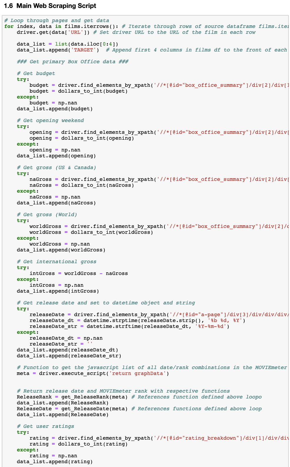
The next phase wasexploratory data analysis to evaluate the distributions, see what correlations there may be between features and if any transformations are needed to better reveal relationships or normalize the data. The first thing is to generate a pair plot of the data. I exclude the one hot encoded genres here both because they are binary values and also for readability:
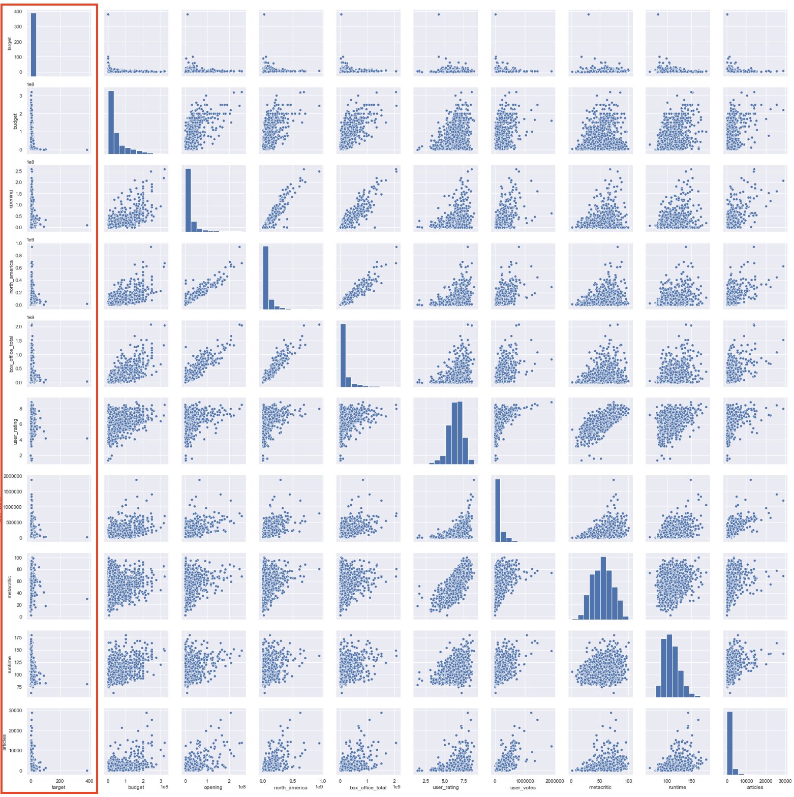
There are some interesting things here and some definite correlations and relationships but some of the data is really hard to parse, especially against the target data, which we are most interested in. Also many of the distributions do not look normally distributed at all. Log transforming the dataframe made the data a bit easier to parse and normalize the data:
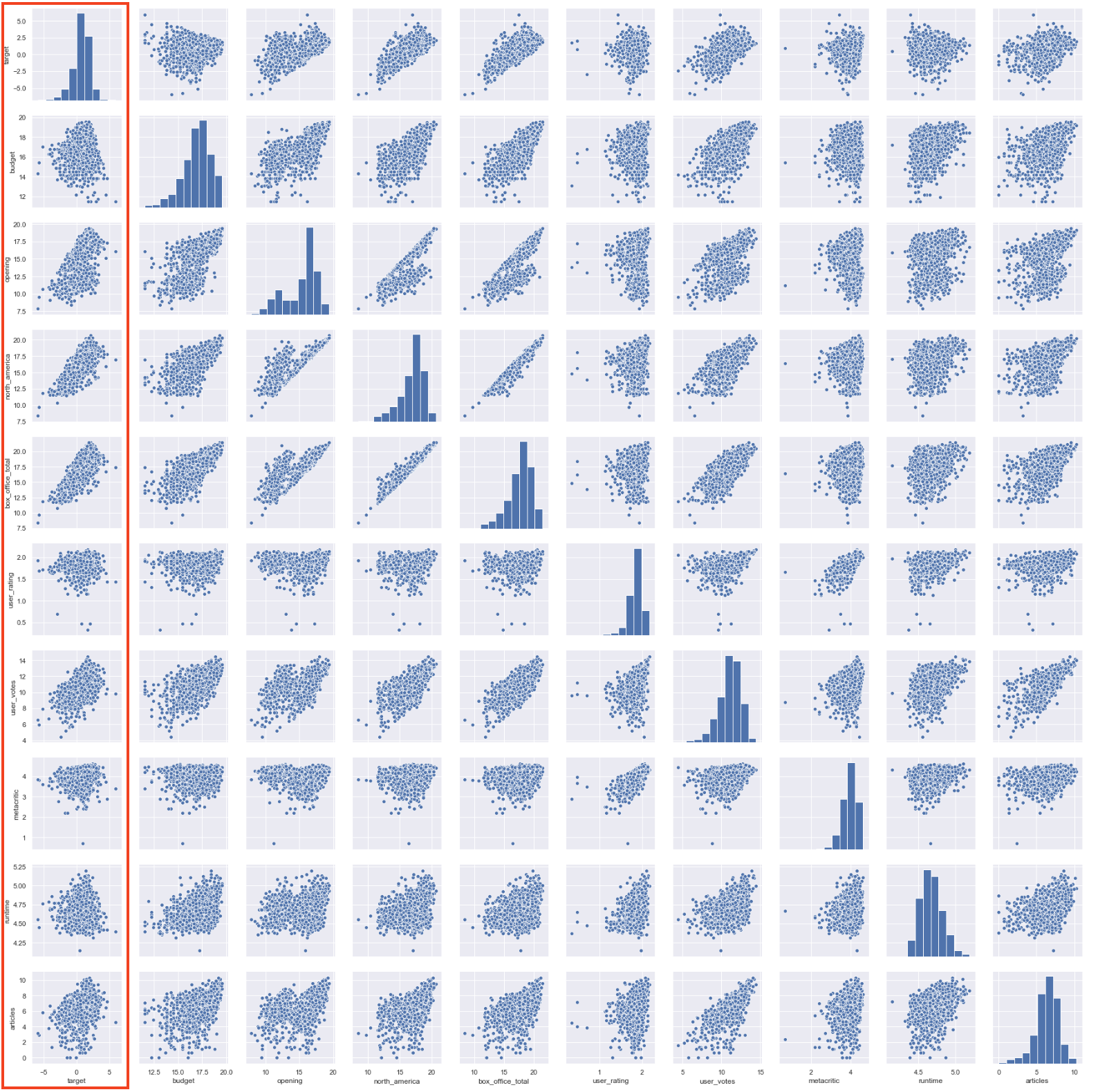
Reducing the number of variables in the pairplot to the variables of interest made some trends clearer as well.
Here we can see that there are relationships between the opening and target as well as possible multicollinearity between box_office_total, opening and north_america.
Additionally it’s worth noting that while the log transform helped normalize the data quite a bit, it could still be better.
Adding Features
Before we get to feature trimming to deal with collinearity, I added some features that I felt were necessary. I actually should have done this before I started pairplotting, but here we are:
- opening_ratio - This is (opening weekend) / (budget), how much of the budget is recouped in the opening weekend. We already have the opening revenue, but it is the proportion of that revenue that recoups the budget that we’re most interested in as a feature.
- na_ratio - This is (North American revenue) / (total revenue). I’m interested in if there is a correlation between the proportion of revenue being generated in North America and the recoup on budget, versus the proportion of international revenue.
- intl_ratio - (International revenue) / (total_revenue). The complement of the ratio above.
Removing Non-International Observations
Adding the intl_ratio actually revealed something useful. There are films where the proportion of revenue from international sales is 0. This means that there was no international release. In total there were 56 of these films. Ultimately I decided to remove these observations, for similar reasons to those mentioned above concerning the target audience for this analysis. Any film of any significant budget will need to pursue an international release, so I don’t want observations that don’t have it. With this the dataset drops from 1475 to 1419 observations.
Yeo-Johnson Transformation to Normalize
While log transformations have improved interpretability and distributions a bit, other power transformations can be even better at revealing relationships and normalizing data. I applied a Yeo-Johnson transformation to the data primarily to attempt to make the data distribution more Gaussian.

While still not perfect, the Yeo-Johnson power transformation seems to have helped normalize the data, at least upon visual examination. We’ll need to do more rigorous tests to see how much it really helped.
Correlations and Multicollinearity
First to deal with the apparent multicollinearity. A heatmap is a simple way to see where there might be problems:
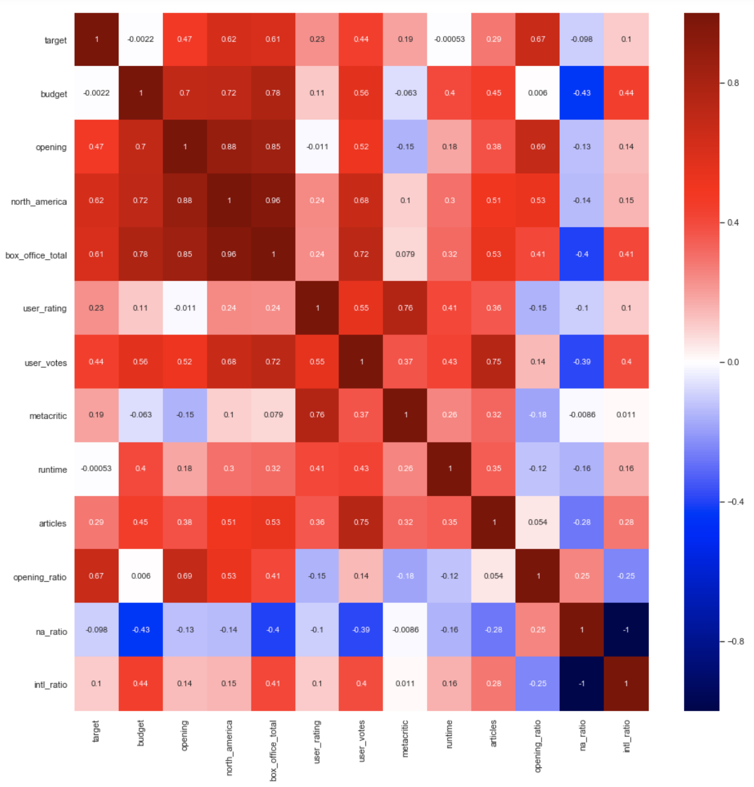
With this kind of heatmap numbers close to 1 or -1 are the ones to look out for. We can see here a few serious contenders:
- box_office_total + (budget, opening weekend, North American revenue): are related (mostly) through box_office_total
- na_ratio + intl_ratio: share the same denominator box_office_total
- Metacritic + user_rating: critics and viewers don’t always agree, but they mostly do, thus we have correlation
- user_votes + box_office_total: the more people who see a movie, the more reviews it’s likely to get
Just about all of these make intuitive sense for the reasons given. We need to figure out how to deal with them, but we also need a metric to decide which ones we need to address and which we can ignore.
Variance Inflation Factor
Variance Inflation Factor measures how much of an effect on variance a particular feature has. The accepted metric is that any feature with a VIF over 5 should be looked at. As usual scikit-learn has a function that can calculate it:
budget                17.239848
opening               29.474925
north_america        146.926679
box_office_total     155.213017
user_rating            4.096932
user_votes             6.875463
metacritic             2.899722
runtime                2.148405
articles               2.602439
opening_ratio         14.845208
na_ratio            2984.784036
intl_ratio          2805.339912
This data correlates with what we saw in the heatmap. When we have multicollinearity it essentially means that we have two or more features that are giving the same information, so we’ll want to eliminate features so that only one is providing that information. Ultimately I decided to remove opening, na_ratio, intl_ratio, north_america and box_office_total for the reasons given below.
- opening: factor of opening_ratio
- na_ratio: box_office_total is a factor
- intl_ratio: box_office_total is a factor
- north_america: box_office_total is a factor
- box_office_total: factor of opening_ratio
All of these features are actually of interest to me and I may use them in a different study of this data, but for the purposes of this analysis we can do without them. After removing those features these are the VIF scores we are left with:
budget            3.742150
user_rating       4.028306
user_votes        5.346148
metacritic        2.808896
runtime           2.126532
articles          2.514226
opening_ratio     1.346704
Action            2.074713
Adventure         2.214139
Animation         1.940845
Biography         1.397190
Comedy            2.392119
Crime             1.390039
Documentary       1.428846
Drama             2.387433
Family            1.276517
Fantasy           1.345215
History           1.198842
Horror            1.758833
Music             1.153554
Musical           1.021830
Mystery           1.366026
Romance           1.430263
Sci-Fi            1.437750
Sport             1.120821
Thriller          1.664611
War               1.042119
Western           1.038359
A much better result. We’ll go with dropping the features mentioned above. Our final variables (including genres) are:
['budget',
 'user_rating',
 'user_votes',
 'metacritic',
 'runtime',
 'articles',
 'opening_ratio',
 'Action',
 'Adventure',
 'Animation',
 'Biography',
 'Comedy',
 'Crime',
 'Documentary',
 'Drama',
 'Family',
 'Fantasy',
 'History',
 'Horror',
 'Music',
 'Musical',
 'Mystery',
 'Romance',
 'Sci-Fi',
 'Sport',
 'Thriller',
 'War',
 'Western']
Evaluate Distributions
Next I evaluate the distributions to see how Gaussian they are. That data is Gaussian is very important for many statistical tests and models, including linear regression. We’ll use both the Shapiro-Wilk and D’Agostino-Pearson tests.
Shapiro-Wilk Test Results
         Features  Statistics  P-Values                   Normal
0          target       0.994     0.000           NO (Reject H0)
1          budget       0.993     0.000           NO (Reject H0)
2     user_rating       0.998     0.029           NO (Reject H0)
3      user_votes       0.998     0.183  YES (Fail to Reject H0)
4      metacritic       0.995     0.000           NO (Reject H0)
5         runtime       0.996     0.000           NO (Reject H0)
6        articles       0.996     0.001           NO (Reject H0)
7   opening_ratio       0.960     0.000           NO (Reject H0)
D'Agostino and Pearson's Test Results
         Features  Statistics  P-Values                   Normal
0          target       3.490     0.175  YES (Fail to Reject H0)
1          budget       9.250     0.010           NO (Reject H0)
2     user_rating       0.016     0.992  YES (Fail to Reject H0)
3      user_votes       2.926     0.232  YES (Fail to Reject H0)
4      metacritic      30.856     0.000           NO (Reject H0)
5         runtime       1.398     0.497  YES (Fail to Reject H0)
6        articles       6.619     0.037           NO (Reject H0)
7   opening_ratio     125.704     0.000           NO (Reject H0)
The D’Agostino test is more encouraging than the Shapiro-Wilk, though both are much better after Yeo-Johnson transformation than before. Before transformation all distributions failed for both tests. Moving forward we’ll have to bear in mind that the distributions aren’t totally normal when drawing conclusions about the models.
Linear Regression Models
And now we finally get to the modeling work. We’ll be using both StatsModels and scikit-learn. StatsModels has great statistical data, but is somewhat limited in terms of tools for splits, validation and regularization.
StatsModels Ordinary Least Squares Regression
Simply running StatsModels’ standard Ordinary Least Squares (OLS) regression yielded these results:
                            OLS Regression Results
==============================================================================
Dep. Variable:                 target   R-squared:                       0.691
Model:                            OLS   Adj. R-squared:                  0.685
Method:                 Least Squares   F-statistic:                     111.1
Date:                							 --   Prob (F-statistic):               0.00
Time:                        			 --   Log-Likelihood:                -1179.7
No. Observations:                1419   AIC:                             2417.
Df Residuals:                    1390   BIC:                             2570.
Df Model:                          28
Covariance Type:            nonrobust
=================================================================================
                    coef    std err          t      P>|t|      [0.025      0.975]
---------------------------------------------------------------------------------
Intercept        -0.0545      0.074     -0.737      0.461      -0.199       0.090
budget           -0.3892      0.029    -13.499      0.000      -0.446      -0.333
user_rating      -0.0233      0.030     -0.780      0.435      -0.082       0.035
user_votes        0.6105      0.034     17.715      0.000       0.543       0.678
metacritic        0.0436      0.025      1.744      0.081      -0.005       0.093
runtime           0.0251      0.022      1.155      0.248      -0.018       0.068
articles         -0.0262      0.024     -1.110      0.267      -0.073       0.020
opening_ratio     0.5835      0.017     33.739      0.000       0.550       0.617
Action           -0.0904      0.047     -1.936      0.053      -0.182       0.001
Adventure         0.2282      0.051      4.452      0.000       0.128       0.329
Animation         0.4696      0.079      5.971      0.000       0.315       0.624
Biography         0.2302      0.059      3.934      0.000       0.115       0.345
Comedy           -0.0034      0.048     -0.072      0.942      -0.097       0.090
Crime            -0.2351      0.048     -4.913      0.000      -0.329      -0.141
Documentary       0.2924      0.133      2.201      0.028       0.032       0.553
Drama            -0.0392      0.046     -0.852      0.394      -0.130       0.051
Family            0.2614      0.071      3.684      0.000       0.122       0.401
Fantasy          -0.0218      0.061     -0.357      0.721      -0.141       0.098
History           0.0951      0.089      1.074      0.283      -0.079       0.269
Horror            0.0380      0.065      0.585      0.559      -0.090       0.166
Music             0.1415      0.089      1.582      0.114      -0.034       0.317
Musical           0.1755      0.201      0.872      0.383      -0.219       0.570
Mystery          -0.0064      0.061     -0.105      0.917      -0.127       0.114
Romance           0.0881      0.052      1.705      0.088      -0.013       0.189
SciFi            -0.1680      0.063     -2.684      0.007      -0.291      -0.045
Sport            -0.3285      0.120     -2.739      0.006      -0.564      -0.093
Thriller          0.0341      0.051      0.665      0.506      -0.067       0.135
War              -0.2006      0.173     -1.156      0.248      -0.541       0.140
Western          -0.3503      0.191     -1.831      0.067      -0.726       0.025
==============================================================================
Omnibus:                       57.304   Durbin-Watson:                   1.961
Prob(Omnibus):                  0.000   Jarque-Bera (JB):               74.731
Skew:                           0.410   Prob(JB):                     5.92e-17
Kurtosis:                       3.769   Cond. No.                         24.2
==============================================================================

Warnings:
[1] Standard Errors assume that the covariance matrix of the errors is correctly specified.
We’ve got an ok R-Squared/Adjusted R-Squared of 0.691/0.685. Was hoping for better prediction, especially given that some of this data is post-release data, but this may be as good as we get. This is before we do any kind of cross-validation, testing or regularization, which can all reduce the R-Squared.
There are also some p-values of note for the features (user_rating, runtime, metacritic, articles, and an assortment of genres). Perhaps they aren’t very predictive. When we get to regularization we’ll see if this can be confirmed.
Also of note are the residuals on the prediction. They imply that the residuals aren’t normally distributed, which can be an issue:
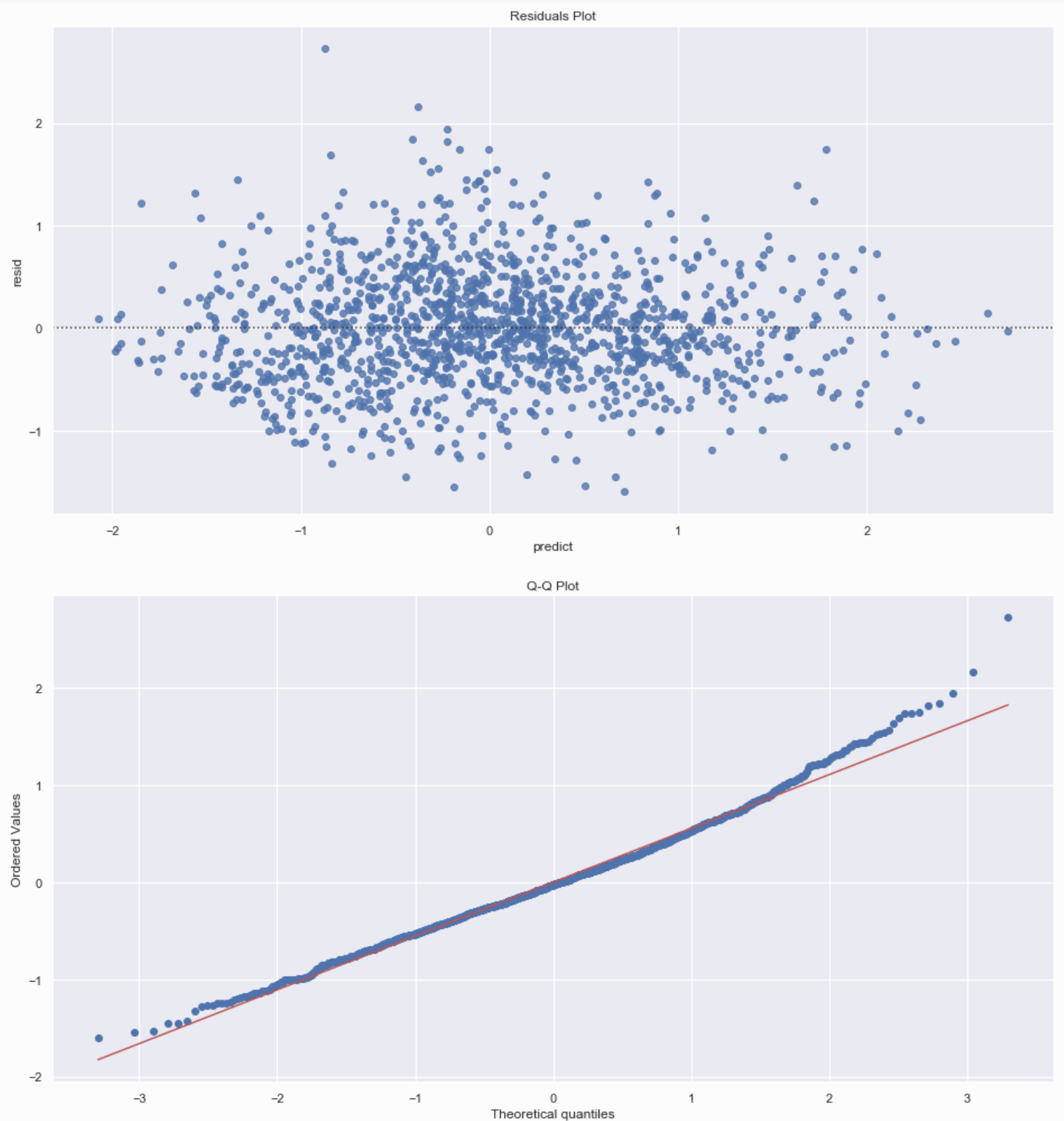
Shapiro-Wilk Test Results
Statistics: 0.99, P-Value: 0.0
Data does not look normal (Reject H0)

D'Agostino/Pearson Test Results
Statistics: 57.304, P-Value: 0.0
Data does not look normal (Reject H0)
Huber-White Linear Regression
Huber-White regression, is supposed to be robust to outliers so we hope that it will yield a better result in terms of the residuals distribution:
Huber-White Regression
R2 Score: 0.6836

Shapiro-Wilk Test Results
Statistics: 0.975, P-Value: 0.0
Data does not look normal (Reject H0)

D'Agostino/Pearson Test Results
Statistics: 128.638, P-Value: 0.0
Data does not look normal (Reject H0)
However, it does not appear to have helped. The distribution of residuals is still not completely normal. As such we’ll proceed with Ordinary Least Squares. While we can see some hetero scedasticity in the plot, it doesn’t appear to be so dramatic that it will ruin the results.
Split and Validate
We’ll use scikit-learn to split and validate the model. We split and validate to make our model more generalizeable so the scoring results drop less on test.
Validation R2 Score: 0.6860340533782777
Feature Coefficients:

budget : -0.41
user_rating : -0.01
user_votes : 0.59
metacritic : 0.05
runtime : 0.04
articles : -0.03
opening_ratio : 0.59
Action : -0.03
Adventure : 0.31
Animation : 0.32
Biography : 0.11
Comedy : 0.07
Crime : -0.25
Documentary : 0.35
Drama : 0.01
Family : 0.18
Fantasy : 0.01
History : 0.14
Horror : 0.05
Music : 0.16
Musical : 0.07
Mystery : -0.02
Romance : 0.09
SciFi : -0.22
Sport : -0.26
Thriller : 0.01
War : -0.26
Western : -0.26
The split and validate R-Squared results are very close to standard OLS in StatsModels: 0.686. Let’s see if we can improve overall performance with interaction terms or polynomials.
Polynomials
In looking at the pairplot of the final variables we can see what seems to be a non-linear relationship between target and opening_ratio.
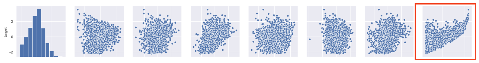
Perhaps taking the square of opening_ratio will improve prediction:
Validation R2 Score: 0.6555111730544533
Again unfortunately it has not, and that was the only feature that seemed like it had polynomial potential. We’ll proceed to cross-validation and regularization with the features as is.
Cross-Validation and Regularization
We’ll now apply both cross-validation and regularization techniques, specifically Ridge and LASSO, to see if we can get better generalizability on test and better interpretability in terms of what features matter most. Also, in addition to R-Squared, we’ll be using Mean Absolute Error (MAE) as a measure of performance. MAE can be a more reliable measure of predictive power as it is looking strictly at the reduction in the cost function, versus R-Squared where it’s numbers can sometimes be deceptive.
Both Ridge and LASSO regularization apply a hyperparameter called Alpha which tunes how strong the regularization effect will be. We want to find the best alpha value that both reduces the effect of strong coefficients, but retains features and coefficients that are valuable for prediction. We’ll use LASSO, Ridge and their cross-validation counterparts to find these optimal Alphas with the lowest MAE.
Lasso Results
LASSO Regularization
Alpha: 0.0023
Mean Absolute Error: 0.4235
R-Squared: 0.7001
Ridge Results
Ridge Regularization
Alpha: 24.37
Mean Absolute Error: 0.4217
R-Squared: 0.7026
LASSO Cross-Validation Results
LassoCV Regularization
Alpha: 0.0133
Mean Absolute Error: 0.4238
R-Squared: 0.7053
Ridge Cross-Validation Test Results
RidgeCV Regularization
Alpha: 5.1497
Mean Absolute Error: 0.4238
R-Squared: 0.7053
So overall, all methods produced roughly the same R-Squared and Mean Absolute Error on test:
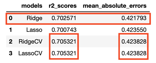
A couple of things to bear in mind here though. One is that RidgeCV and LassoCV have identical scores by both criteria. However, more importan is that the R-Squared of LassoCV and RidgeCV is higher than Ridge even though the MAE of Ridge is lower. So what to do? Due to the potential issues with R-Squared scores when you have to choose between MAE and R-Squared, I’m opting for MAE so the Ridge regularizedl is the final model we’ll go with.
Use Ridge Model on Test Data
Finally we apply the selected model to the test data, which resulted in the following scores:
- R-Squared = 0.6404
- MAE = 0.4573
This is a significant, but not surprising drop in performance on test versus validation. Specifically:
- R-Squared: -0.06
- MAE: +0.03
While we hope that test will be very close to training and validation and we take many steps, such as train-test-split and cross-validation to make sure we don’t overfit on the training data. This is not a shocking performance drop.
Feature Relevance for ROI
And now that we have the best model, what are the coefficients so we can evaluate how important they are for film budget return on investment?
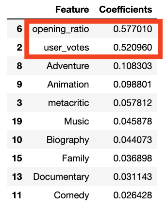
So it seems that by far opening_ratio and user_votes are the most important factors to maximizeto improve return on investment, at least according to this model. It’s interesting that certain genres like Adventure and Animation are more important than Metacritic rating and also that genres seem to matter more than other factors such as user_rating, articles and budget. This is definitely worthy of further exploration in other studies.
Conclusions
- The number of user ratings and the ratio of the opening weekend revenue to total revenue matter the most in terms of improving ROI. This would seem to confirm Hollywood’s obsession with the opening weeked. It does appear to matter a great deal. I think we can look at the number of user ratings as proxy for ticket sales. The more people see a film the more ratings there will be for that film. Pretty simple. As such it probably really isn’t much of a unique predictor.
- Of all of the models attempted the standard Ridge regularization model without cross-validation performed the best. However, that performance is nowhere near as high as we would like, with an R-Squared of only 0.6404.
- These features are rather heavily skewed, which may contribute to their predictive value. We were never able to get the features to look completely Gaussian, despite many transformations.
- There is room for considerable improvement so we should look at additional variables that could produce better results, hopefully focusing solely on data that is available before the film’s release to see what kind of prediction we can generate.
Future Work
- There is a rather important category of predictor that I wasn’t able to use for this study, principal cast and crew. In the future I would like to use data about the popularity of principal cast and crew of a film to see what predictive power it could have for a linear model. Specifically I would like to look at their STARMeter rating before release and the historical financial peformance of films they’ve been in before the release of the film in question. I think there’s great potential for solid prediction with these features.