
Seattle Airbnb Project

1. Project Overview
This is a project that I felt would be relatively simple, but that turned out to be much more involved. While I have done several machine learning projects before this was the first time that I had such a high number of features that I couldn’t practically dive deep on each one individually. This gave me valuable experience in coming up with strategies to deal with large numbers of features and prioritizing the methods to deal with them efficiently, while still maintaining some time constraints for the project.
The goal of this project was to take an Airbnb dataset for all of the properties in Seattle, Washington 2016 and use it to answer 3 questions about the data and then come up with a predictive model for a feature of the data.
Visit the Github repo to see the data, code and notebooks used in the project.
Data
The data consisted of 3 datasets:
- calendar (1.4M rows, 4 columns): Covers listing ids of properties, dates, availability of the property and the daily price of staying at the property.
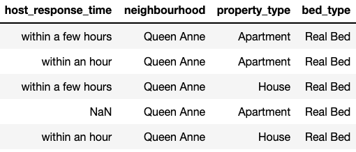
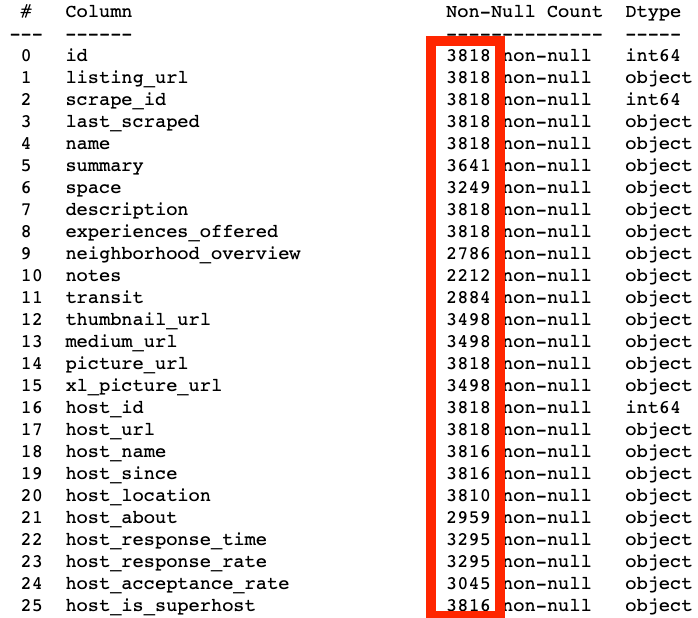
- listings (3818 rows, 92 columns): Covers many aspects of each listing such as descriptions and details of the property and host, review scores, location, amenities, etc.
- reviews (84,849 rows, 6 columns) Focuses on written reviews for stays at each property.
My questions and modeling focused on the property listings, so I didn’t end up using the reviews dataset.
3 Questions to Answer:
- What is the overall occupancy in Seattle over the course of the year?
- Are there periodic shifts in the overall Airbnb occupancy in Seattle over the course of the year and if so what does this look like? This can help the company decide when and how to run promotions of various kinds and to work with hosts to help them get the most out of these time frames.
- Does it pay to be a Superhost? How do the occupancy, prices and reviews of Superhosts compare to normal hosts?
-
Superhost is a special title that is automatically applied to listings where the host maintains high marks in many areas and has an established positive trend with Airbnb overall.
-
I’m interested in seeing if there is a correlation between being a superhost and other metrics, such as overall rating/reviews, occupancy, and rental prices. I’ll compare these same metrics to non-Superhost listings.
-
- What neighborhoods have the highests occupancy rates?
- Knowing where to have a property for an Airbnb residence can be an important decision for hosts to make. Providing that information to them can help hosts be more effective, as well as helping Airbnb know how to focus its promotional efforts.
Prediction: Mean Annual Occupancy Rate
My predictive model will attempt to predict the mean occupancy rate for a given property listing for the year. The independent variables will be details about the listing, primarily from the listings dataset.
Data Processing
It’s often said about 70-80% of an analysts’ time is spent in the data processing phase and that was certainly the case for this project. I’ll cover the highlights.
Data Conversion
Many of the columns with numerical data I wanted to use was in the form of strings “$85.00” and they needed to be converted to floats or integers, which was fairly straightforward. Example here of code I used to do so:
prices = calendar.price.loc[calendar.price.notna()].apply(lambda x: x[1:]).str.replace(',','')
prices_nans = prices.append(calendar.price.loc[calendar.price.isna()]).sort_index().astype('float64')
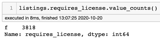
There were also categorical features that where essentially binary values (‘t’/’f’) where I simply replaced those letters with 1 or 0.
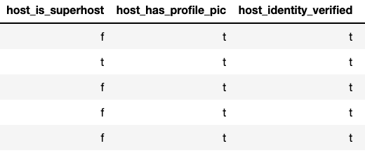
listings.replace({'host_is_superhost': {'t':1, 'f': 0}}, inplace=True)
Categorical Conversion
The most conversion work was that of one-hot encoding multi-category features, a necessary step in preparing categorical variables for modeling, as algorithms can’t use categories in string form. This makes the categories useful, but if there are many categoricals and or many categoricals within them it can explode the amount of features in the dataset, making it more sparse and potentially reducing its predictive power.
In this case doing so increased the number of columns from 92 to over 200, but later on I was able to reduce this number by culling unnecessary columns.
NaN Handling
Dealing with NaNs took up the bulk of the data processing work. The listings dataset had 92 columns to start with varying degrees of NaNs present across many of them.
My approach generally broke down to these approaches:
- Deleting NaN rows where the number of NaNs were extremely low. For this project there were a few that had only a couple of rows with NaNs
- Imputing numerical NaN values.
The main feature where I relied on imputation was host_response_rate, the percentage at which hosts responded to inquiries from guests. There were over 500 NaNs and I didn’t want to use the simple mean or median for such a high percentage (14%) of the data. Instead I created a probability distribution of all of the values based on the counts of each value:
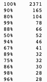
Then randomly assigned one of these values to the NaNs based on the distribution. This was less ideal than regressing the values, but a better solution within the time constraints than just assigning the mean or median to all of the NaN values. Regressing the values would have been its own project and wouldn’t have fit within my time constraints.
Deleting Features
In a number of cases features were simply removed from the dataset:
-
When an extremely high number of observations (99%+) were a single value, making them uninformative from a modeling perspective.
-
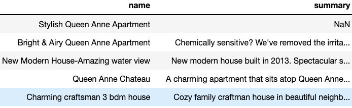
Freeform text fields, as they can’t be easily converted to quantitative values without a lot of NLP work, which would be a project in itself. Often these were feature engineered into features that indicated the length of the string in the observation.
-
When almost all of the observations were NaNs.

3. Feature Engineering
There were a good amount of opportunities for simple feature engineering in this project that ended up being quite useful for the final model. The approaches I took were:
-
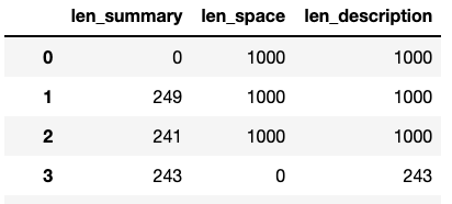
Converting features with freeform text data to numbers that indicated the length of each text field.
-
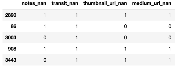
For features with a high amount of NaNs, creating a new feature that indicated whether or not an observation was a NaN. Sometimes NaN/not-NaN observations can constitute their own informative categories.
-
Occupancy rate itself, the target for prediction for the modeling phase, was engineered as the mean of
availablefrom the calendar dataset joined on each listing.
4. Final Dataset
The final dataset I ended up using was the listings dataset with all of the modifications above, and the target, the calculatd annual occupancy rate, added from the calendar dataset. With the encoding of categoricals and dropping of columns and rows the final set had 3816 rows and 148 columns, compared to starting with 3818 rows and 92 columns.
5. Questions to Answer
Q1: What is the overall occupancy in Seattle over the course of the year?
- Are there periodic shifts in the overall Airbnb occupancy in Seattle over the course of the year and if so what does this look like? This can help the company decide when and how to run promotions of various kinds and to work with hosts to help them get the most out of these time frames.
- We’ll look at the mean of all prices each day over the course of the year.
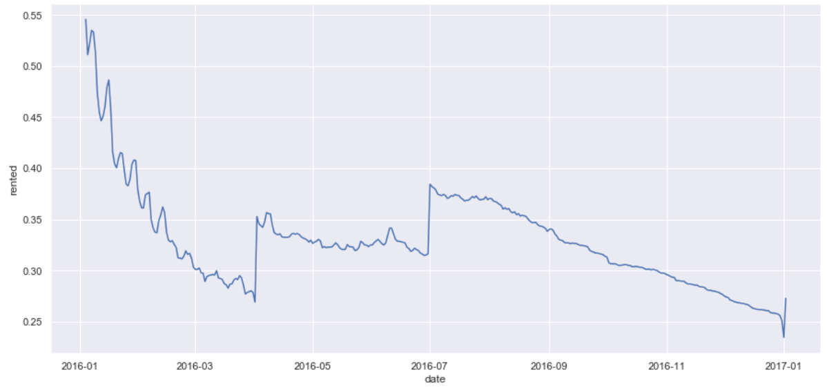
- The trends here are fairly easy to understand. There are three distinct periods where we see a dramatic buildup of reservations followed by a leveling off. We’ll take a closer look at each region.
New Year
- New Year’s would appear to be the time we see the greatest spike in occupancy for Airbnb in Seattle, as occupancy never gets close to that level throughout the rest of the year.
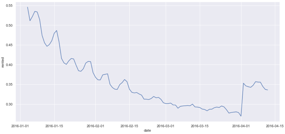
Spring Break
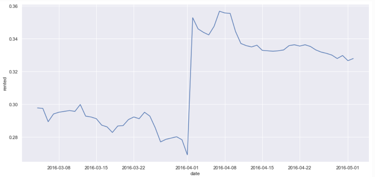
- Looking more closely at the March-April time frame we see a spike around the beginning of April that would seem to correspond to the spring break time frame, which makes sense.
Summer Vacations
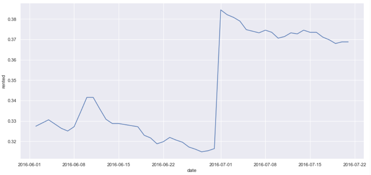
- Again we see an occupancy spike in the June-July time frame, which would correspond with school being out and summer vacations.
Holidays
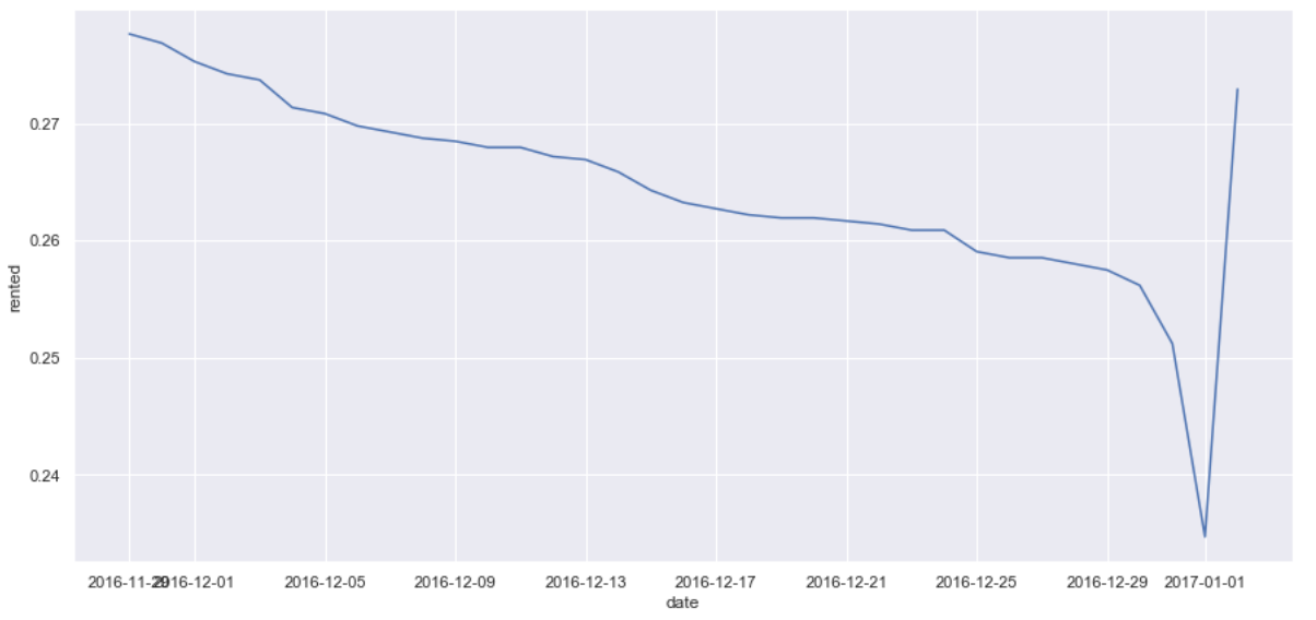
- This last trend is somewhat interesting. The dramatic spike at the end of the year corresponds to New Year’s, but there is a pretty dramatic drop right before then.
Q2: Does it pay to be a Superhost? How do the occupancy, prices and reviews of Superhosts compare to normal hosts?
Superhost is a special title that is automatically applied to listings where the host maintains high marks in many areas and has an established positive trend with Airbnb overall.
I’ll explore whether there is a correlation between being a Superhost and other metrics, such as overall rating/reviews, occupancy, and rental prices to get a better idea if the Superhost program is effective or not for Airbnb.
Occupancy - How do occupancy rates compare between normal hosts and Superhosts?
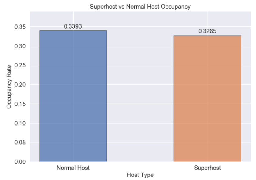
- Interestingly there really doesn’t seem to be much of a difference between normal hosts and Superhosts in terms of their ability to maintain occupancy.
- Occupancy rates are actually slightly higher for normal hosts, but only by about 1.3%. This is somewhat counterintuitive, as you would expect superhosts would be in higher demand.
- This may call into question the efficacy of the Superhost program, but this is only one means of evaluation. Others may reveal advantages for Superhosts.
Average Rental Price - How does average rental price compare between host types?
Given that occupancy rates are roughly the same for both host types, maybe average price of rentals is different between them and this is an area where Superhosts gain an advantage.
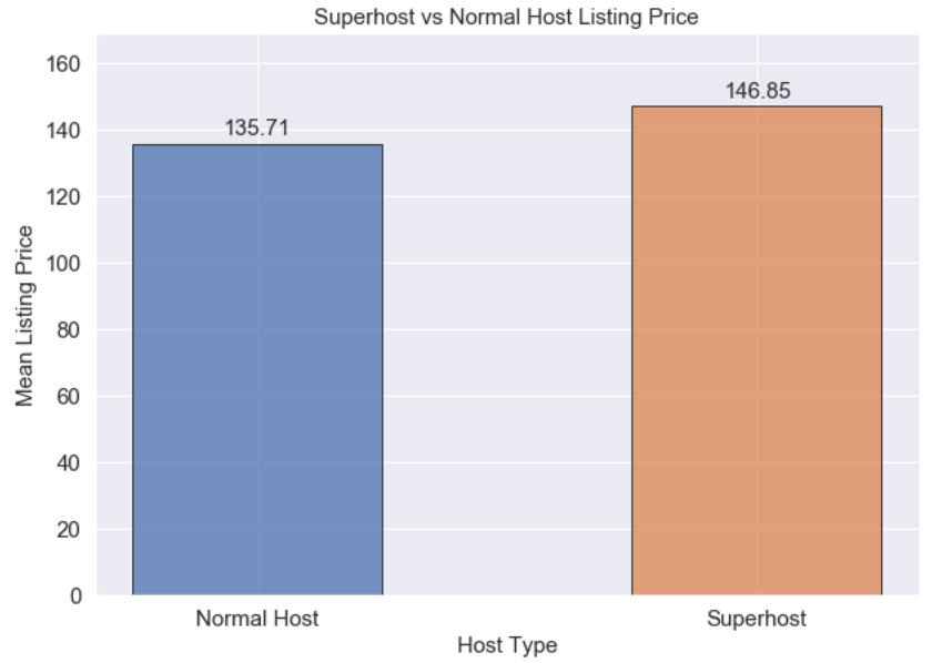
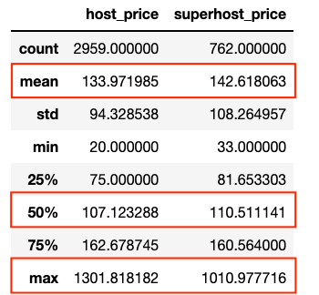
- Here we see a distinct advantage for Superhosts. While the Superhost rental rate is slightly lower than normal hosts (-1.3%), the mean prices for their listings is about 8.2% higher.
- This alone might make striving for Superhost worth the effort. We should also look at the distribution of the prices. Perhaps the center of the distribution is indeed higher or outliers may be driving the average price up.
Listing Price Distribution - How does the distribution of prices for the two hosts’ listings differ?
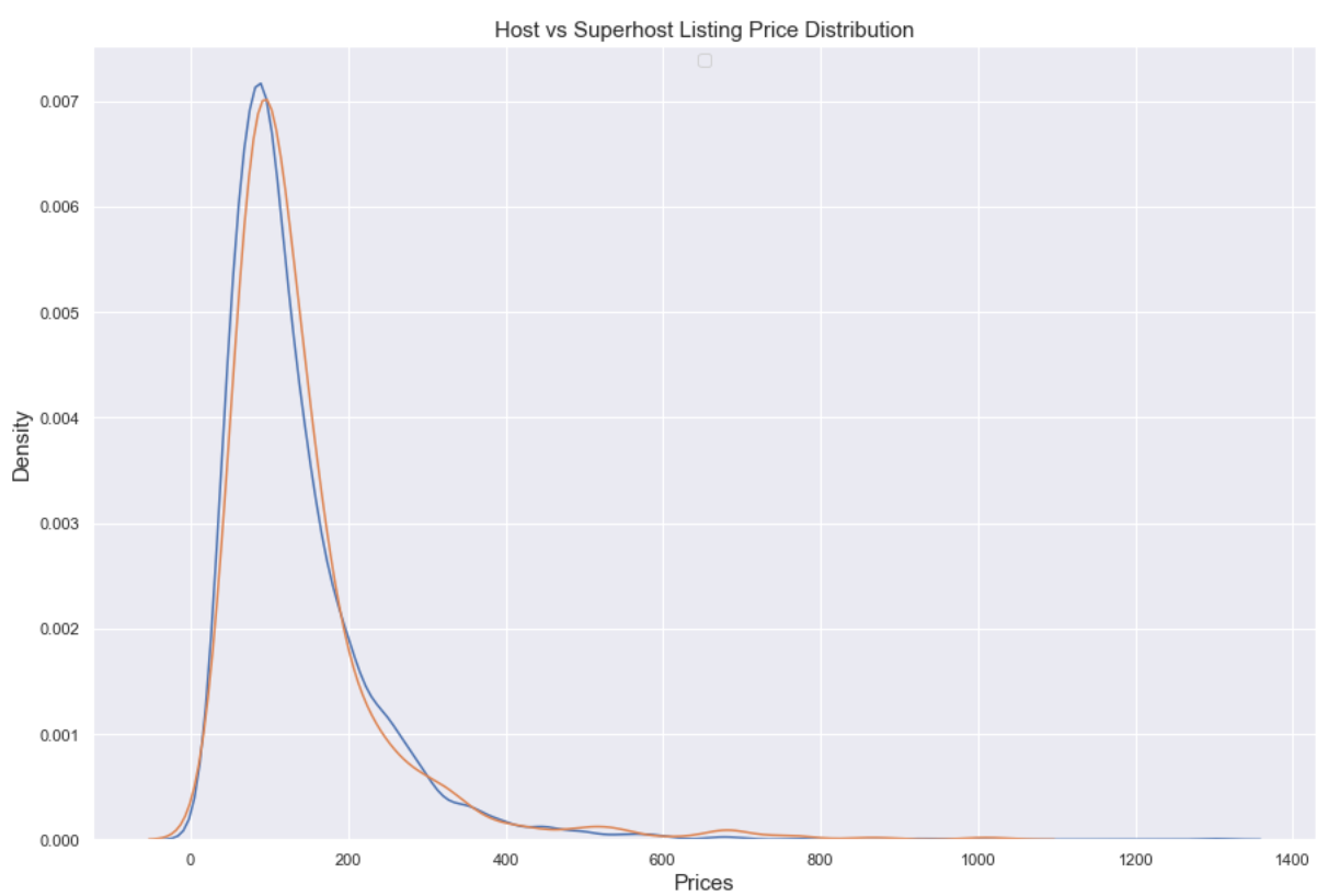
-
This KDE distribution makes them look about the same. Looking at a box plot and descriptive statistics may make things clearer.
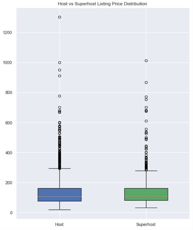
- The occupancy rates of Superhosts and hosts are very close to each other, within about 1%, with the occupancy rate of normal hosts being slightly higher.
- However, the mean price of a Superhost listing is notably higher than that of a normal host, about 8% higher, as we saw before.
- In examining the distributions of prices, the higher mean listing price for Superhosts does not seem attributable to outliers skewing the metric. The distributions prices of both groups are very close, with normal hosts actually having more outliers than Superhosts.
- It seems Superhosts tend to earn more with their listings than normal hosts so it may indeed be worth it to attempt to achieve that status. This would be a good area for further study.
Q3: What neighborhoods have the highest occupancy rates?
Knowing where to have a property for an Airbnb residence can be an important decision for hosts to make. Providing that information to them can help hosts be more effective, as well as helping Airbnb know how to focus its promotional efforts.
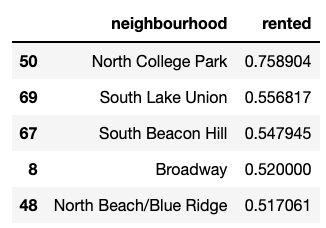
Here are the occupancy rates for each of the 81 neighborhoods:
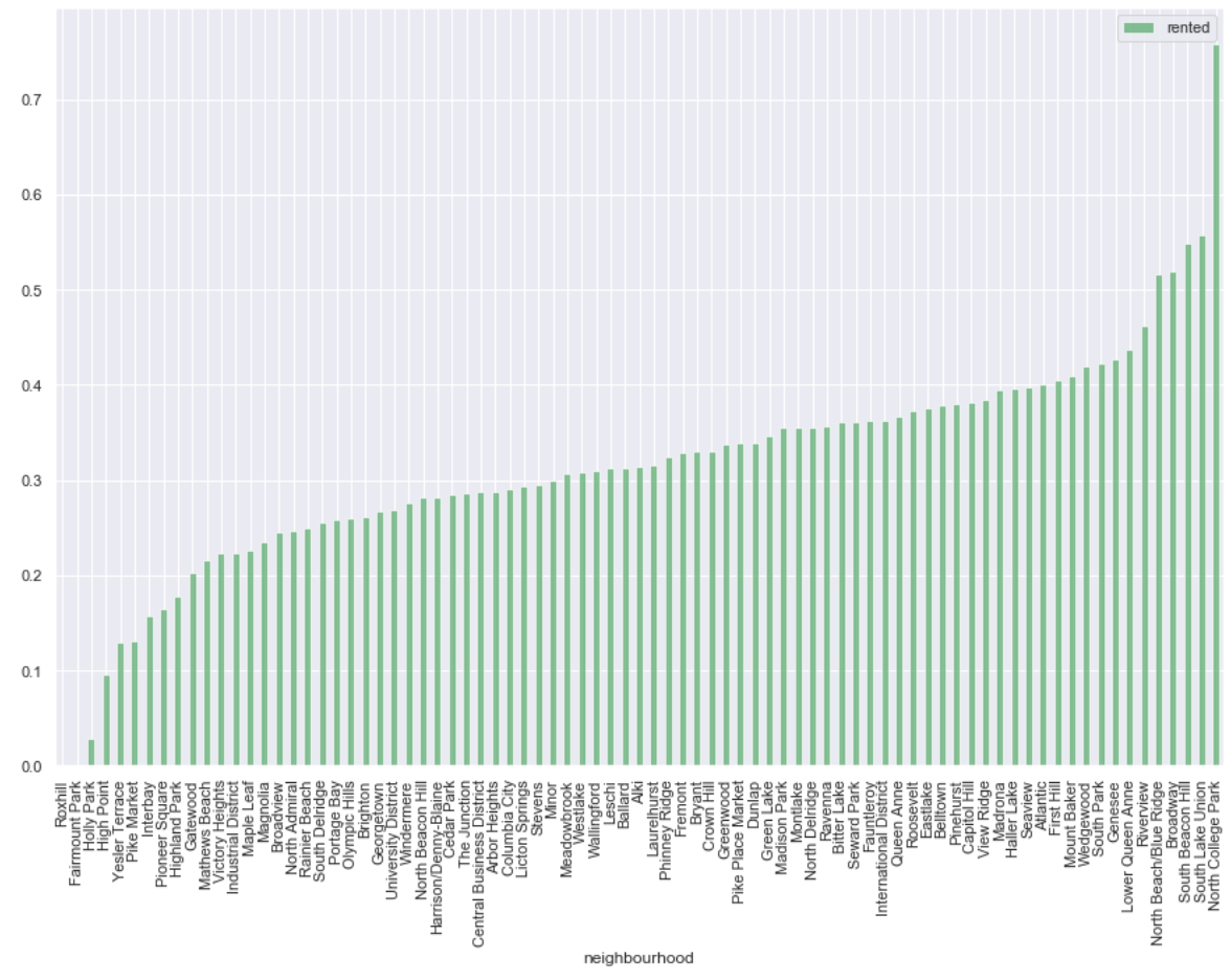
- While most are clustered in the 20-40% range there are clear examples of much higher and much lower occupancy.
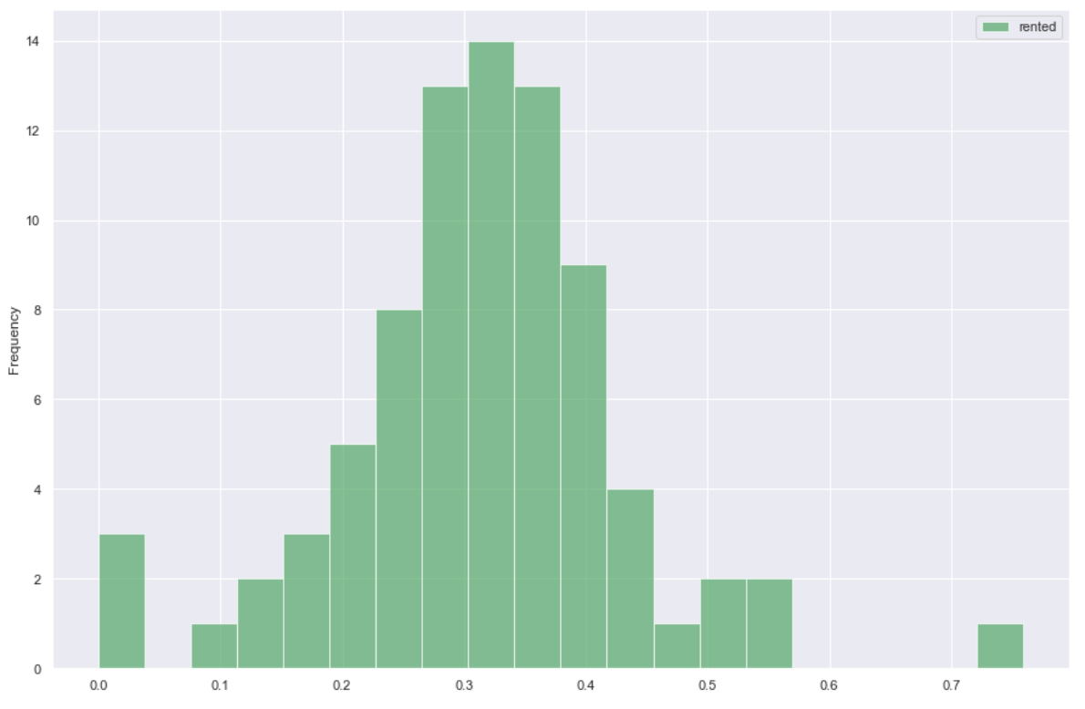
- This histogram clarifies the distribution a bit with lower and higher performers standing out as outliers. However, overall the distribution of occupancy rates seems to be fairly normal.
Highest Occupancy Neighborhoods
There’s not a standard way to define the “top occupancy” so we’ll look at the plots to see where there is a distinct spike for the top performers. This seems to be the spike to over 50% occupancy, which would be the top 5 neighborhoods. This also corresponds to around the 95th percentile of occupancy.
Price vs Occupancy
Pricing may be a factor in occupancy so it would be good to see what the relationship is between occupancy and mean price of a listing.
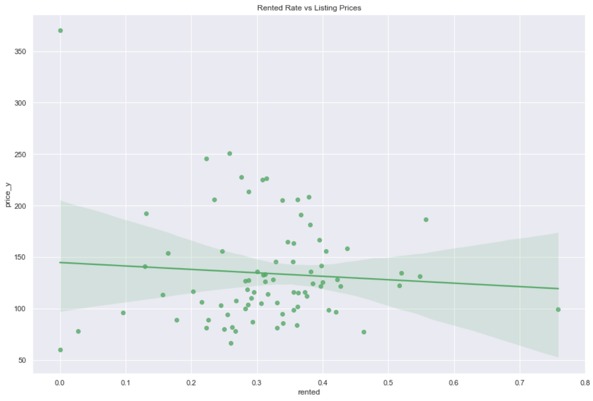
- This scatterplot and regression line strongly indicates there is no relationship between occupancy and listing price. The regression line is almost flat and the distribution of points looks relatively random.
Key Questions: Conclusions
- What is the overall occupancy trend in Seattle over the course of the year?
- There are three distinct periods where we see a dramatic buildup of reservations followed by a leveling off: spring break, July 4th/early summer, and New Year’s.
- The New Year’s spike is the largest and there is a dramatic drop right before New Year’s.
- New Year’s is the time we see the greatest spike in occupancy for Airbnb in Seattle, as occupancy never gets close to that level throughout the rest of the year.
- Does it pay to be a Superhost? How do the occupancy, prices and reviews of Superhosts compare to normal hosts?
- The occupancy rates of Superhosts and hosts are very close to each other, but the mean price of a Superhost listing is notably higher than that of a normal host, about 8% higher.
- The higher mean listing price for Superhosts does not seem attributable to outliers skewing the metric.
- Base on this preliminary analysis it appears that Superhosts tend to earn more with their listings than normal hosts, so it may be worth it to attempt to achieve that status. Further study is needed however.
- What neighborhoods have the highest occupancy rates?
- The specific neighborhoods with the highest occupancy are:
- North College Park
- South Lake Union
- South Beacon Hill
- Broadway
- North Beach/Blue Ridge
- This is useful information to have, as it can be the basis for further exploration into specific details of these neighborhoods that leads to their occupancy rates, but that is outside the scope of this analysis.
- We have per neighborhood occupancy clustering around 30% over the course of the year with some clear outliers on the high end and low end. So there is definitely a difference between different neighborhoods in terms of occupancy, but most hover in the 20-40% range.
- The histogram indicates that neighborhood occupancy is relatively normally distributed.
- There seems to be no relationship between neighborhood occupancy and listing price.
- The specific neighborhoods with the highest occupancy are:
6. Modeling
The modeling process ended up being the most straightforward step. The goal was to create a model that can best predict the annual mean occupancy rate of a particular listing for Airbnb listings in Seattle.
As the target is a continuous numerical variable this is a regression problem so I used a number of regression algorithms to approach it:
- Ridge Regression
- Lasso Regression
- Support Vector Regression
- Random Forest Regression
Scaling
Distance-based algorithms like linear regression and KNN need the numerical values to be standard scaled so the different scales of each variable don’t contribute to skewing the model. I used Scikit-learn’s StandardScaler for this.
Random forest and other tree-based techniques don’t require this, but it also won’t hurt them either, so I stuck with the scaled version of the dataset throughout the modeling process.
Scoring Metrics: Mean Squared Error, Fit Time
Using the mean squared error of the model predictions is fairly standard for this type of regression modeling so I used that as the primary metric.
In addition I also kept track of the fit time. Processing efficiency can be a critical factor in deciding what model to use, so I wanted to bear this in mind when evaluating these models.
Cross-Validation
Cross-validation is always necessary in my mind, in order to increase generalizability of models on test so I used it for every model. Technically random forests are robust enough without it though.
GridSearchCV
I used the GridSearchCV function with each algorithm to search through hyperparameters to find the optimum values.
Baseline: Mean Occupancy Rate
Establishing a baseline is important in order to effectively gauge how much better the trained models are performing. If it can’t outperform a simple baseline significantly it is not a very good model. For this I used Scikit-learn’s DummyRegressor function, which will predict some simple value for all observations.
In this case I used the default prediction of the mean of all occupancy rates, which in this case was 0.3291.
| Metrics | Baseline |
|---|---|
| Mean Squared Error | 0.1178 |
Ridge Regression
Ridge regression applies a regularization on linear regression that penalizes high variance coefficients, effectively reducing bias and overfitting, which can help with generalization of a model to novel data.
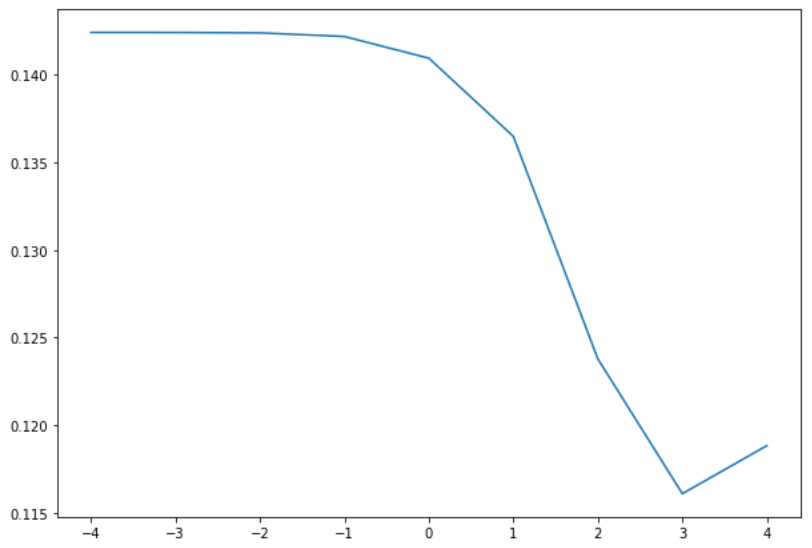
For Ridge (and Lasso) the parameter to be tuned is alpha, and it determines how strongly regularization is applied. I searched through the alpha values [0.0001, 0.001, 0.01, 0.1, 1.0, 10.0, 100.0, 1000.0, 10000.0] initially:
-
The plot above shows the
alphavalue on the x-axis and the mean squared error (MSE) on the y-axis. Note that the x-axis is on the log10 scale. The cross-validation results were:Metrics Ridge Mean Fit Time 0.0205 Best Alpha 1000 Best Mean Squared Error 0.1161 -
This MSE score is better than baseline but only very slightly. It is only a 1.4% improvement over baseline.
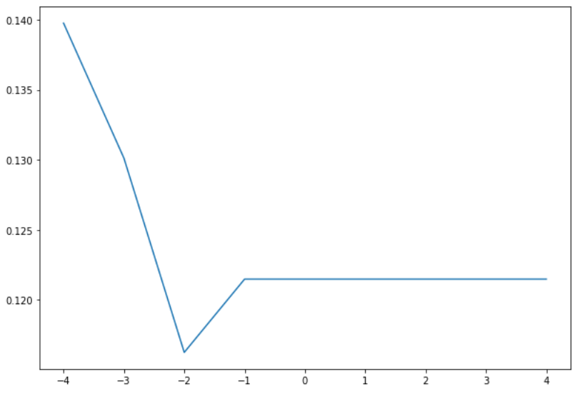
Lasso Regression
Lasso is very similar to ridge regression, except that instead of reducing the effect of feature coefficients it can completely remove features from the model, so lasso is a form of feature selection as well as a regularization method.
Lasso also uses alpha as it’s hyperparameter and I searched over the same set of values as ridge.
| Metrics | Lasso |
|---|---|
| Mean Fit Time | 0.0222 |
| Best Alpha | 0.01 |
| Best Mean Squared Error | 0.1162 |
MSE and fit times are essentially the same between lasso and ridge. Neither is a significant improvement over baseline. I could have continued trying to get incremental improvements here, but it is generally better at this point to try other methods to see if basic modeling with them will yield better performance.
Support Vector Regression
Support vector machines are very flexible due to their implementation of kernels which can fit various types of patterns in the data. Each kernel has different hyperparameters that can be tweaked, but I stuck with default values for the initial investigation of each.
Instead of exhaustively going over each I’ll just present the results:
| Metrics | Linear | Poly | RBF | Sigmoid |
|---|---|---|---|---|
| Mean Fit Time | 28.3864 | 10.3691 | 11.3146 | 13.4671 |
| Mean Squared Error | 0.1689 | 0.3533 | 0.1107 | 269.1618 |
RBF is the clear winner here, though it is, again, only slightly better than baseline. I went on to use GridSearchCV to further explore RBF values and perhaps get a better score. It’s worth noting that the sigmoid kernel is astoundingly bad, somehow generating an error that is completely off of the scale of the target values.
RBF GridSearchCV
The RBF kernel has two hyperparameters gamma and C. C is the equivalent of alpha in lasso/ridge, and applies regularization to the model. gamma determines how much an individual observation influences the overall model.
Instead of searching across both parameters simultaneously, which GridSearchCV is very capable of doing, I searched each parameter individually and then combined them. This ended up generating the best results for SVM.
| Metrics | SVM (RBF) |
|---|---|
| Mean Fit Time | 1.8697 |
| Best C | 1 |
| Best Gamma | 0.1 |
| Best Mean Squared Error | 0.1084 |
SVM with the RBF kernel has generated the best MSE so far: 0.1084. The fit time is significantly worse than lasso and ridge, though.
Random Forest Regression
Random Forests are an ensemble modeling method that takes several weak learners, decision trees, and combines their results to make predictions.
Random Forests have many more hyperparameters than SVM or OLS methods, but the two that are the most important are the number of decision trees (n_estimators) and the number of features (max_features). I focused on these in my searches.
I applied the same approach as I did with SVM RBF. I found the best value for each parameter individually then combined them.
| Metrics | Random Forest |
|---|---|
| Mean Fit Time | 7.8555 |
| Best Estimators | 1300 |
| Best Feature Selection | square root |
| Best Mean Squared Error | 0.0992 |
This is the best MSE of all of the models I produced: 0.0992. This is a 15.62% improvement over baseline.
It is also the slowest to fit. This fit time is not a huge concern for this project, but it could be for a much larger dataset and model when you try to put it into production.
Test with Best Model
Random forests performed the best so I tested the held out testing data to see what score it could get on prediction. Generally, it’s not unusual to see a massive drop in performance when going from training to testing, but that fortunately was not the case here.
| Metrics | Random Forest Test |
|---|---|
| Mean Fit Time | 6.8459 |
| Estimators | 1300 |
| Feature Selection | square root |
| Test Mean Squared Error | 0.0994 |
This is surprisingly excellent performance on test with an MSE of 0.0994, compared to 0.0992 on validation. This is a loss in performance of only 0.2%, which is pretty impressive, considering how much performance can normally drop.
Feature Importances
Random forests allow us to see the relative importance of each features, which is often the thing we are most interested in with a project.
Top 20 Features
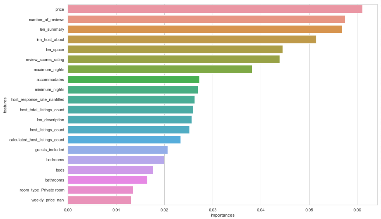
- This is pretty insightful. Unsurprisingly price is the most important factor in terms of occupancy rate, so pricing competitively will likely lead to better outcomes, though we would need to investigate what the actual relationship with pricing is.
- It’s good to see that a number of the engineered features are amongst the most important. Lengths of descriptions alone seem to be a factor in occupancy. Likely the longer your description the higher the chance that your property will be rented.
- The imputed host response rate (host_response_rate_nanfilled) is in the top 10 features in terms of importance, so that was a good feature engineering effort to put in. Generating the NaN binary categorical for weekly price turned out well also.
- Other features that are unsurprisingly important are the number of listings for the host, and the number of beds, bedrooms and bathrooms.
Bottom 20 Features
Seeing the bottom 20 features can be helpful as well.
<img src=”/images/airbnb_seattle_project/Screen Shot 2020-10-20 at 5.03.43 PM.png)
- These results are similarly insightful and interesting. Amongst the features of the lowest importance are many of the neighborhoods. Though I suspect these are the neighborhoods that have the lowest occupancy, the fact that neighborhoods are not in the top 20 reinforces that they perhaps aren’t a major factor in determining whether or not a property is occupied.
- Also property types of various kinds are either low importance or low priority.
7. Modeling Conclusions
- In the end random forests had the best model performance of all of the modeling techniques tried. Random forests tend to perform quite well on more complex modeling tasks, so this isn’t terribly surprising. It also generates useful outputs like feature importance, which can be a very important component of a project.
- We ended up with a final mean squared error on test of 0.0994, which was ~15.62% better than baseline and only 0.2% worse than validation, which means that the model is likely highly generalizable to new data with the same features.
- While random forests did generate the best model in terms of predictive power, it was the worst in terms of performance. This is not a major concern for this project, but must always be considered.
- In terms of feature importances many of the engineered features ended up being in the top features in terms of relevance to the model. This shows how important feature engineering can be to a project.
- While I did explore a number of algorithms and dug in on a few, there are many more that could be employed and we could go much deeper on techniques of optimizing, refining and combining them to get even better performance.
8. Resources
- GitHub Repository - GitHub repository containing all code, notebooks and data.