1. Proposal

This project focuses on natural language processing (NLP) and unsupervised learning to look at movie reviews and attempt to analyze them using these methods. Specifically, I wanted perform sentiment analysis on the reviews to gauge the overall positive or negative valence of the review and then perform topic modeling to see what topics are prominent for the negative reviews.

Looking at a number of movies would provide a lot of data with which to perform training and analysis, but I felt it the more generalized insights would not be as interesting as focusing on a single film. When you analyze a number of movies, segregate by review valence then topic model you discover a number of topics for reviews that are positive, neutral, and negative towards all of these movies. This could be useful, but I felt it was more academic than a case study of one film, where you could potentially get more specific topics.

When you look at one film then you (hopefully) get much more fine-grained detail about topics specific to that film and thus deeper insight. Coming from the games industry, which has a number of strong parallels to the film, what content creators are interested in is the consumer response to our product, both while it is in development and after it is released. Having consumer insight helps us to understand what is important to them and can help guide the creative process to make sure we are making a product that they will find compelling. These insights also help inform our public relations and social media response to consumer concerns. When we can get to the core of the overall trends in consumer opinion we craft effective messaging in publicly responding to it.

The film I chose for this project was Star Wars: The Last Jedi. There are a number of reasons why I settled on this film. First, Star Wars is a massive pop culture franchise, perhaps the largest in existence, so it is a film of great relevance for understanding popular opinion, and also there would be no shortage of data to work with. Second, The Last Jedi is objectively the most divisive Star Wars film ever. The original trilogy of films is generally universally liked by the fanbase and the “Prequel” film trilogy is generally disliked, but The Last Jedi has split fan opinion in two. The negative voices tend to be the loudest on social media and YouTube, but there is also a great deal of positive support for the film as well, with many calling it their favorite Star Wars film. Never has opinion on a film in this franchise been so divided, so it felt like a good one for evaluating consumer opinion.

Additionally, the concept of “toxic fandom” is a prominent one amongst creators of entertainment content in general, but especially for movies and games. Negative reviews of The Last Jedi extended beyond critiques of the film content itself and dove into socio-political commentaries around feminism, racism, social justice warriors (SJWs) and related topics. One actress in film was driven off social media due to the toxic nature of the negative backlash. There was even a study done to investigate whether the strong negative response was agenda-driven or even part of a Russian influence operation.

Regardless of whether or not this was the case though, while toxic fandoms usually represent a small percentage of the most engaged part of fan communities, which themselves are a small percentage of overall consumers, fan communities pour disproportionate time and energy to driving the conversation around a piece of content, to the point where they can sway public opinion. As such the opinion of fandoms as well as the general public are of even greater interest when they turn toxic. These trends are top of mind for content creators so having a method to understand the conversation in aggregate would be very useful for them.

So with this in mind, I will first perform a sentiment analysis on reviews of Star Wars: The Last Jedi then perform topic modeling on the negative reviews to see what issues are of most concern to those who did not like the film.

Visit the Github repo to see the data, code and notebooks used in the project.

Assumptions

• The most important assumption for this film is that the online written reviews of the film represent a good sampling of actual opinions coming from each main sentiment valence: positive, neutral, negative
• However, from the standpoint of distributions, we will assume that negative reviews are disproportionately represented in the written reviews, which we will be focusing on for topic modeling. It’s generally accepted the consumers, especially on the internet, pour more energy into negative opinion than neutral or positive opinion. This works in our favor in terms of getting a variety of negative opinions and since that’s what we’re interested in, not uniform class distributions, the imbalance shouldn’t affect the analysis.

Methodology

• Use unsupervised learning tools in NLTK and the Google Cloud Platform Natural Language API to perform sentiment analysis of reviews of The Last Jedi and use this to assign a sentiment valence of each review of positive, neutral, or negative.
• Use unsupervised learning techniques, Latent Dirichlet Allocation (LDA) and Non-Negative Matrix Factorization (NMF) to perform topic modeling on the negative reviews of the film and discover the main topics of concern for those who left negative reviews.

Data

• The data consisted of 5865 written reviews was web scraped from the [written reviews page of IMDb](https://www.imdb.com/title/tt2527336/reviews?ref_=tt_ov_rt “IMDb - Star Wars: The Last Jedi User Reviews).
• The data was scraped using a combination of BeautifulSoup and Selenium.
• Both the written review and the user-submitted score for the movie were scraped. The score was used as a rough test for the accuracy of the sentiment valence.

2. Tools

• Python
• Jupyter Notebooks
• Pandas
• Numpy
• Seaborn
• Matplotlib
• Scikit-learn
• BeautifulSoup
• Selenium
• Regular Expressions
• Gensim
• NLTK
• Google Cloud Natural Language API

3. Web Scraping

Source File: imdb_web_scrape.py

Web scraping for this project was fairly straightforward. The reviews needed to be scraped from the [written reviews page of IMDb](https://www.imdb.com/title/tt2527336/reviews?ref_=tt_ov_rt “IMDb - Star Wars: The Last Jedi User Reviews) for The Last Jedi. All of the reviews can be displayed on one page, but the initial search only serves up 25 reviews. A button at the bottom of the page needs to be pressed to serve up additional reviews and each press gives 25 more reviews. With all of the reviews present we then need to extract the review text and the numerical score.

I used Selenium to login to IMDb, go to the reviews page and press the “Load More” button repeatedly until all reviews were revealed. The total was 5865 reviews, which required over 200 automated presses. Brute force, but about the only way to get at all of the reviews when working with IMDb review pages.

I then used BeautifulSoup to parse the pages and extract the written review text and numerical review score. During the extraction process I was able to use regular expressions to deal with the HTML tag content. Getting the numerical scores required a bit of work with regular expressions to make sure I was getting the right number. I also had to deal with missing scores to which I assigned a NaN value.

Interestingly, it’s possible to leave a full review on IMDb and not a review score. Around 300 of the reviews did not have scores, a surprisingly large number. I would need to decide how to deal with these when performing sentiment analysis.

After the scraping was complete I had a dataframe with two columns, one for the review and the other for the review score.

4. Sentiment Analysis

Source File: Sentiment_Analysis.ipynb

Additional pre-processing of the text was needed to prepare it for sentiment analysis. I used regular expressions to remove numbers, lower case all words and remove punctuation. I also used regex to remove egregiously misspelled words (“aaaaaanywaaays”) or nonsense words consisting only of repeated letters (“zzzz”, “zzzzzzz”, etc.) and change score numbers from strings to numbers. I did not yet remove stop words, as I wanted to see what the results were with minimal preprocessing first.

First step was to tokenize the text, which I did using word_tokenize from NLTK. I added this as the third column in my dataframe to try to keep all of the content together.

My first sentiment analysis pass was with NLTK’s built-in sentiment analysis tool, SentimentIntensityAnalyzer(), which produced the following results:

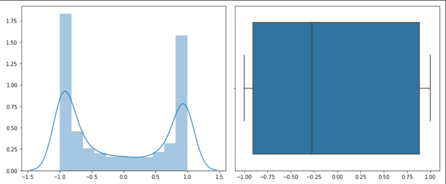
However, these aren’t as informative in isolation. They could be very accurate, very inaccurate or somewhere in between. Under normal circumstances with unsupervised learning you don’t have some ground truth for comparison, as that is what makes it unsupervised, but in this case we can actually compare, since we have review scores in addition to the reviews themselves. However, to keep it high level we’ll just be comparing distributions, to see how close NLTK gets to the “shape” of the actual reviews:

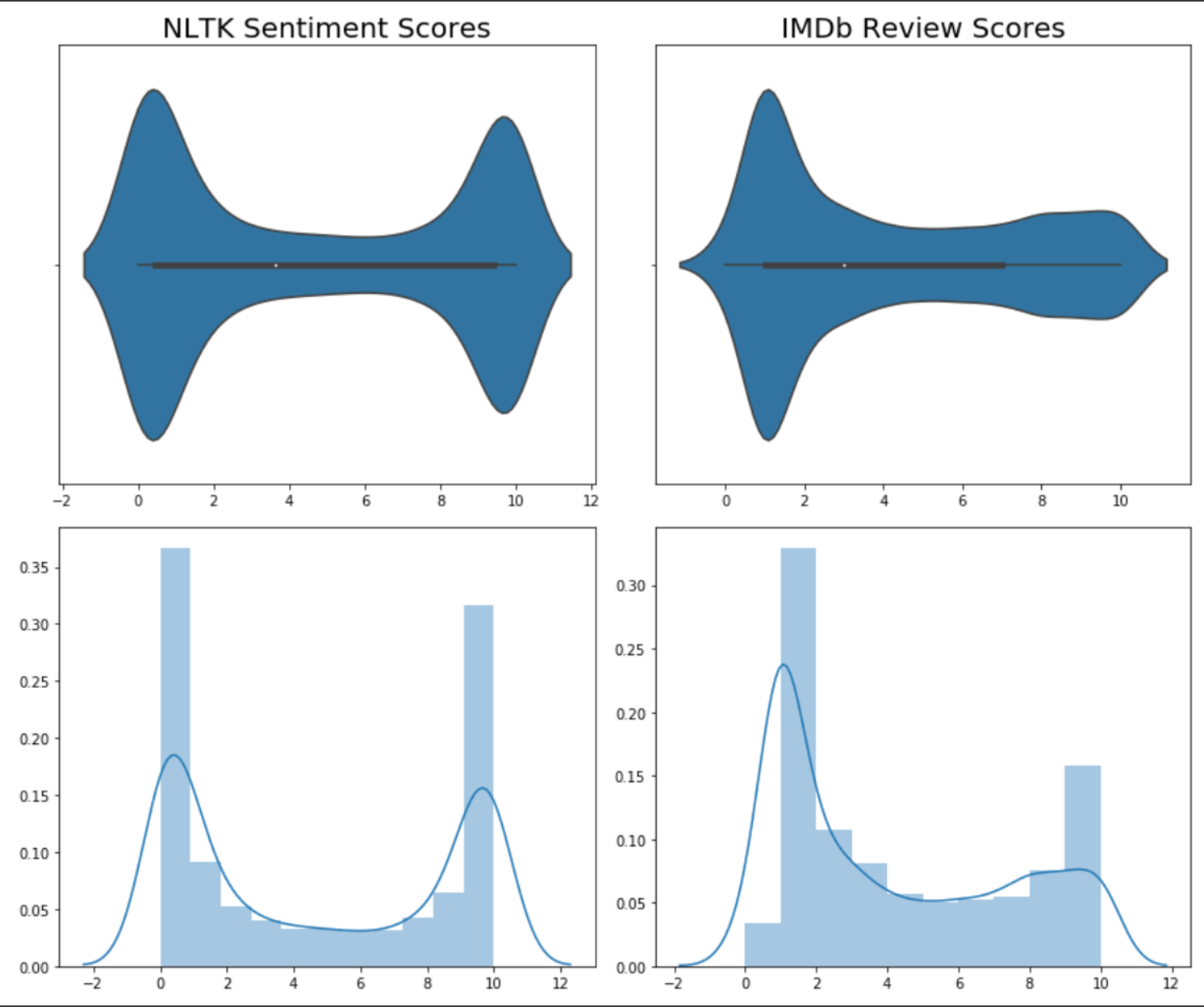
This gives a much better idea of how NLTK compares to IMDb. Here we are comparing the distributions of scores between the NLTK estimate and the IMDb “truth”. What we can see here is that the NLTK scores are far more bimodal than the IMDb scores, which are much more negatively skewed. This gives us a hint that there is significant room for improvement.

One thing to bear in mind however, is that the IMDb score is based on a numerical value that a user inputs, whereas the NLTK score is based on the estimate of sentiment from the review text, so this is not a direct comparison and thus the validation through the IMDb score is a little fuzzy. For the purposes of the analysis though I will assume that a user is fairly accurately representing their review text through their numerical score. It is their quantification of their own feelings that are expressed through the review text.

Next I assigned a review valence to each review for both IMDb and NLTK scores based on the score:

• IMDb Scores
  • 0 - 4 = “Negative”
  • 5 - 6 = “Neutral”
  • 7 - 10 = “Positive”
• NLTK Scores
  • 0.00 - 4.50 = “Negative”
  • 4.51 - 6.99 = “Neutral”
  • 7.00 - 10.0 = “Positive”

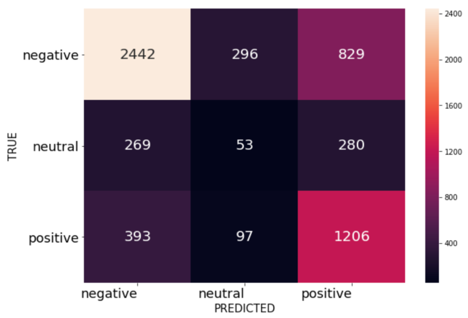
Then I put these two distributions into a confusion matrix to get a more detailed look at the recall accuracy of NLTK. My focus here was exclusively on recall, as I was mostly interested in getting the negatives that are there than making sure that the negatives actually are negatives.

NLTK Sentiment Analysis

• Negative recall: 0.6846
• Overall recall: 0.6310

These were not stellar numbers for recall, so there was definite room for improvement.

Next I looked at the Google Cloud Platform Natural Language API. This API provides a number of services, but the one I was interested in was their sentiment analysis tool. When you feed it text it returns both a sentiment score on a range of -1 to 1 (negative to positive) and a magnitude score indicating the estimated strength of that sentiment. After signing up for a Google Cloud account you get a free year with many of the tools of the service and $300 worth of credits for the tools when you go beyond free allotments. The pricing seems very reasonable with 5000 free text analyses per month and $1 per additional 1000 analyses. When working on mid to large scale games or film this is a minuscule cost.

While not a perfect fit, the results from the Google API were more promising, at least with the goal of topic modeling negative reviews:

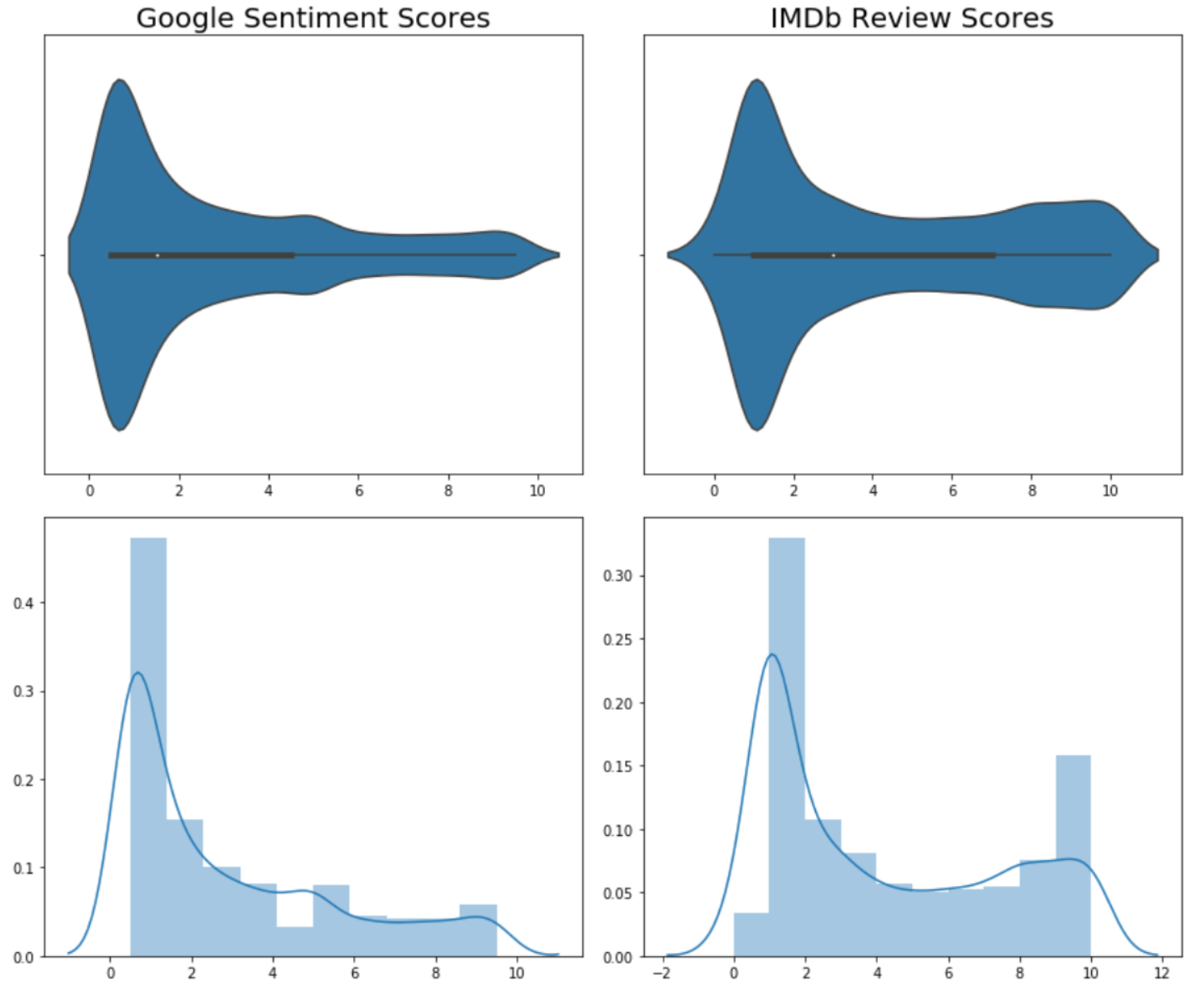
Above we can see that the distribution shape of the Google sentiment scores are closer to the IMDb scores than the NLTK scores. We’ll compare all 3 here:

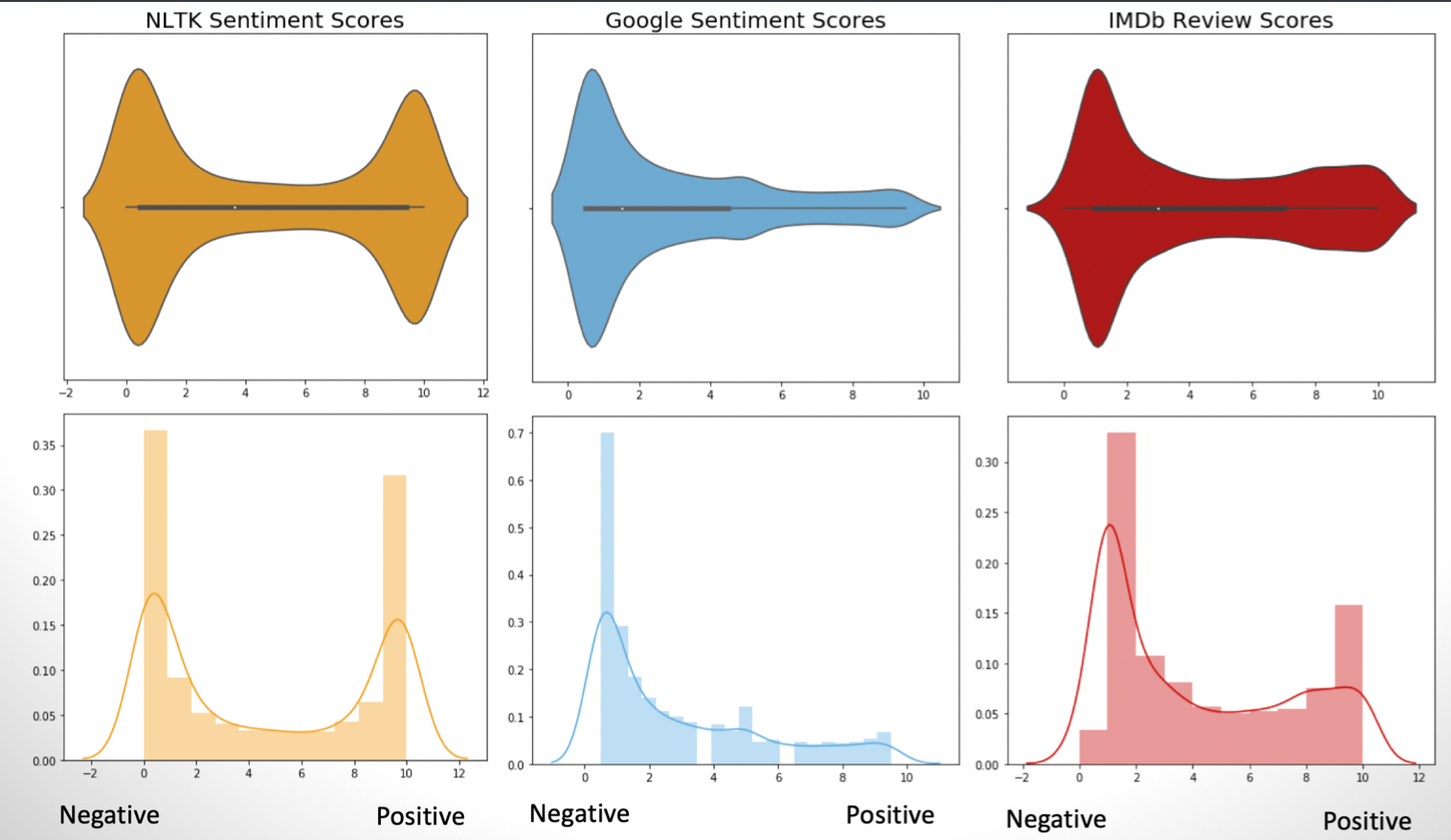
While Google is definitely more negatively skewed than all of the distributions, it is a bit closer to the IMDb distribution, especially in terms of the negative reviews. We see this in the recall scores on from the confusion matrix:

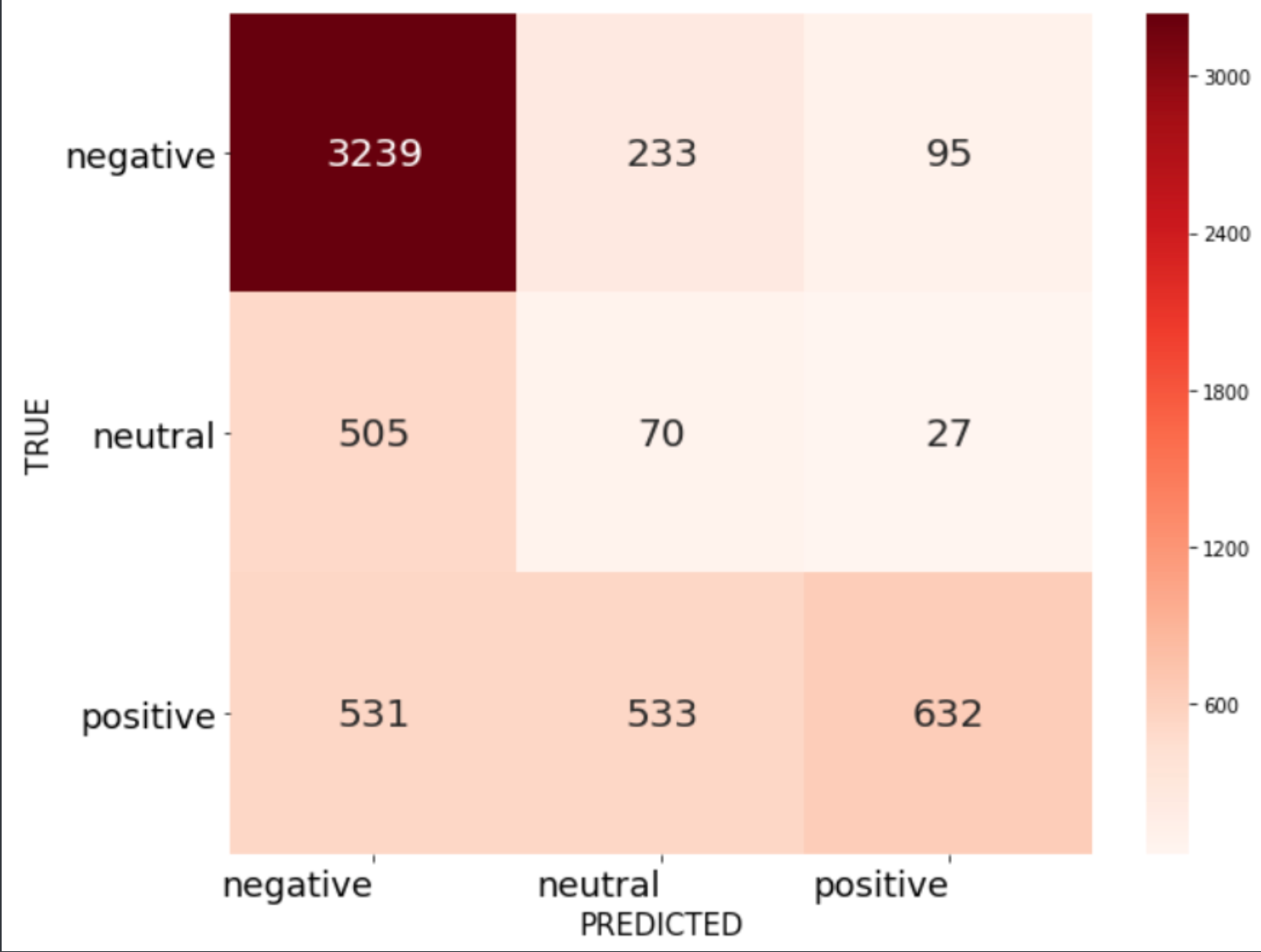
Google Cloud Natural Language Sentiment Analysis Tool

• Negative Recall: 0.9080
• Neutral Recall: 0.1163
• Positive Recall: 0.3726
• Overall Recall: 0.6719

We can see here that the recall is excellent for the negative reviews, which also brings up the overall recall, though to be fair, the recall for the other two categories is pretty abysmal. But because we’re primarily concerned with the negative reviews this is a better than NLTK.

Naive Bayes Classifier

I also took a stab at training a Naive Bayes classifier using NLTK’s Naive Bayes module. However, the accuracy rating was only around 0.5697, which is worse than both the NLTK sentiment analysis tool and Google’s result.

Sentiment Analysis Conclusion

In the end Google’s Cloud Platform’s Natural Language API performed best for identifying negative reviews. It definitely underperformed for the other categories, but since negative reviews are the target this its classification method is the one I went with. A few things to note:

• Google Cloud’s NLP tools have an “Auto ML” function as well that allows you to use Google’s tools to train your own model. This could be a promising next step in the future to improve results across the board.
• Additional tweaking of the corpus (stop words, lemmatization, etc.) could probably have yielded better results across the board. Definitely another area to explore in the future.
• We’ll have to take into account that within the topic modeling we may be getting some topics related to neutral or positive reviews due to the significant amount of false positives in the negative category.

5. Topic Modeling

Latent Dirichlet Allocation (LDA)

Source Files: LDA Code

Source File: Gensim LDA Topics & Visualization Notebook

Source File: Scikit-learn LDA Topics & Visualization Notebook

With the valence labels established, I proceeded to topic modeling on the negative valence reviews. I started with Latent Dirichlet Allocation (LDA) with the Gensim library and tried many different approaches.

To prepare the data I removed English stopwords using NLTK and pulled out the tokenized reviews into a list, which will form the basis of the bag-of-words corpus for our LDA approach. I then created both bigrams and trigrams, lemmatized the text keeping only nouns, adjectives, verbs and adverbs, and created the final corpus and dictionary using Gensim functions.

I then created the first LDA model with 20 topics using the lemmatized bigrams version of the corpus. I calculated the perplexity and coherence of this first attempt for the negative-only reviews:

• Perplexity: -9.972
• Coherence: 0.4657

Perplexity and coherence aren’t normalized values though. They only really matter when compared to other perplexity and coherence scores. However, this can serve as a baseline. Below are some of the topics:

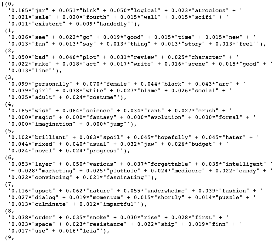
There are some somewhat intelligible topics like Topic 0 addressing the type of humor in the movie and Topic 3 seeming to talk about socio-political topics. As for the main point of interest though, it was difficult to pull definitive meanings from these results.

I also looked at them with a very useful visualization from pyLDAvis that shows a 2D representation of the groupings of the words. Note that the topics above are zero-indexed whereas pyLDAvis starts at 1.

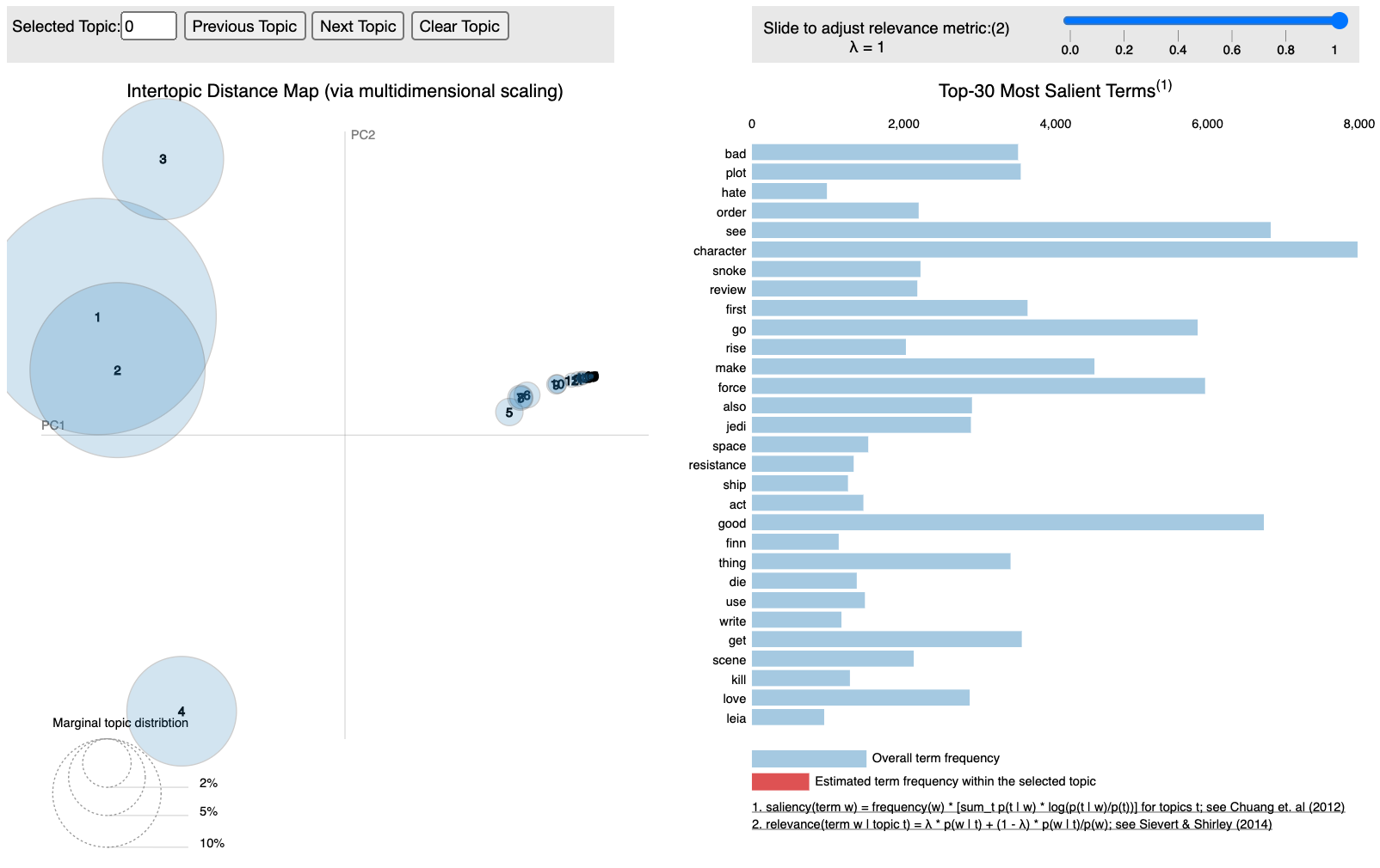
We can see that there is significant overlap between topics 1 and 2, slight overlap with Topic 3, then significant separation on Topic 4. The rest of the topics are of much smaller relevance and overlap strongly. Ideally we would want to see topics of similar size with good separation between them, so this is a far from ideal distribution.

Iterate Through Topic Values

Rather than using trial and error manually, I decided to try use a function to find the optimal number of topics and other parameters for this data set. This function would iterate through different topic numbers and attempt to find the optimal number of topics for the model, with coherence as the main metric:

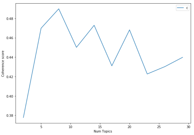
• Top Coherence Score: 0.4898
• Optimal Topic Number: 8

However, after plugging in 8 to the model though the results were actually worse in terms of topic intelligibility and plot separation:

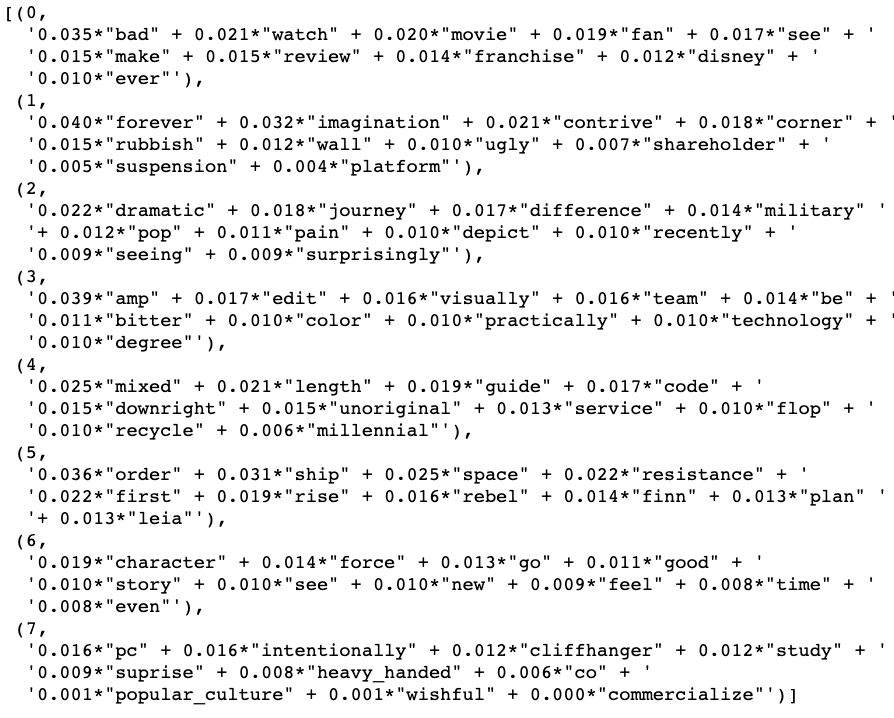
The topics are far more generalized, with little in terms of a distinct idea emerging from the terms.

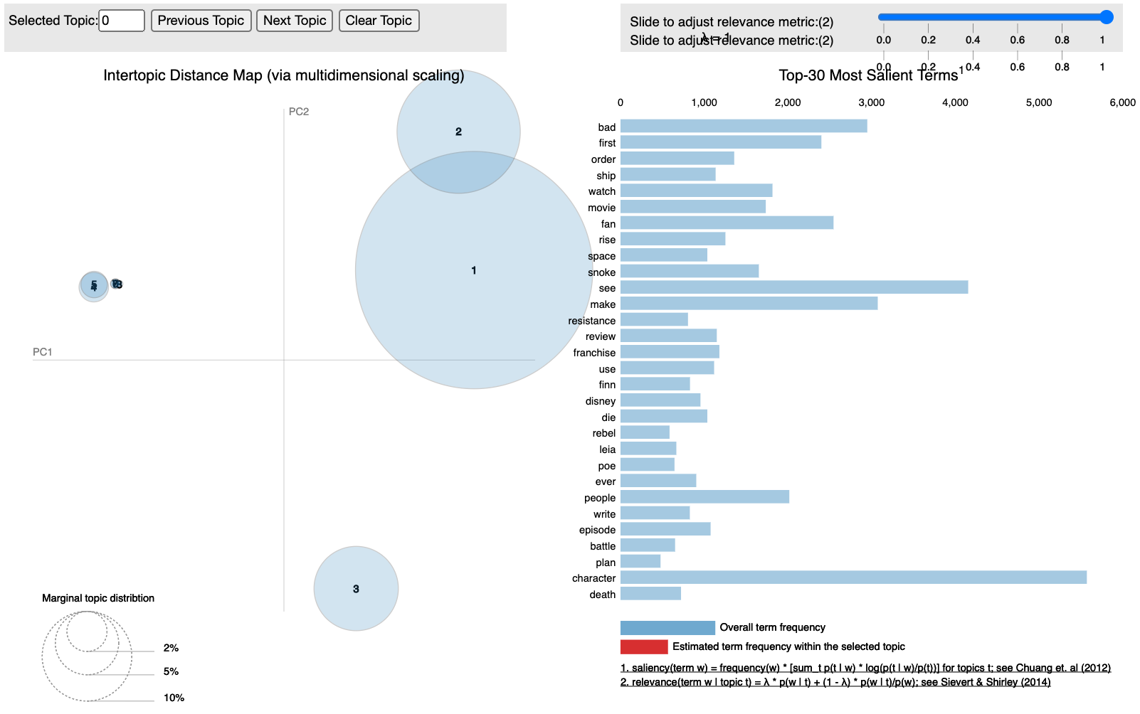
This is further reflected in the pyLDAvis plot, which has only 3 somewhat distinct topics, but that are comprised of a disproportionate amount of the terms. Also, the remaining topics show severe overlapping.

GridSearch with scikit-learn

To do a more comprehensive search for optimum values I used GridSearchCV and the scikit-learn package version of LDA. To do so I had to use CountVectorizer() to turn the data into a sparse matrix and then set both topic numbers (5-40, 5 step) and learning decay values (0.5, 0.7, 0.9) to iterate through. This search ended up not yielding more intelligible results.

It’s important to note that scikit-learn uses log-likelihood as a scoring metric for LDA, whereas we were using coherence as the main metric in gensim. This in addition to whatever differences there are in the LDA implementation in scikit-learn and gensim could also lead to differences in results.

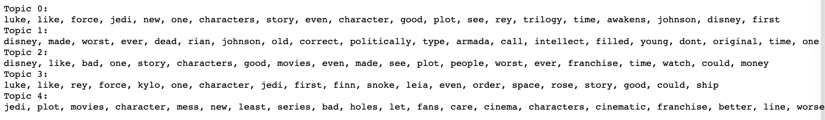
The optimum results for GridSearchCV with LDA was 5 topics and a learning decay of 0.5. However, while these 5 topics had somewhat better separation on the plot, they were completely useless for discerning topics. They were just far too general:

Since the model chose the lowest possible topic value in the GridSearch (5 out of 5 - 40), I wanted to do another search pass to see if it would just keep choosing lower and lower values. I did another GridSearch focusing on a lower start point and smaller range (2-30, 2 step) and again LDA chose the smallest topic number, 2. This seems to imply that there is something strange going on with the model in general or it’s just having a terrible time with this dataset.

At this point LDA was just not working out so I decided to try something else, Non-Negative Matrix Factorization (NMF) .

Non-Negative Matrix Factorization (NMF)

Source File: NMF Code

Source File:NMF Topics & Visualization Notebook

Non-negative matrix factorization ended up being a much easier and more effective approach to topic modeling for this project. As with LDA I removed stop words and lemmatized the data. I used Term Frequency-Inverse Document Frequency (TF-IDF) to prepare the data for the model.

I then iterated through different topic values (5, 10, 15, 20). Note that this was not any iteration algorithm like GridSearch, but running the algorithm individually on the different topic values.

NMF does not have built-in quantitative metrics to evaluate performance, so evaluation was based largely on a subjective evaluation of the topics alone. The LDA modeling experience made me less confident about quantitative metrics for this project so not having a quantitative measure didn’t really bother me. However, pyLDAvis visualization did continue to be useful for at least reinforcing these evaluations.

As for these different topic values, as I increased the number of topics their intelligibility increased as well. I ended up going with 20 topics, as it seemed to generate the most intelligible topics, at least for 1-gram keywords. Below is a selection of those topics

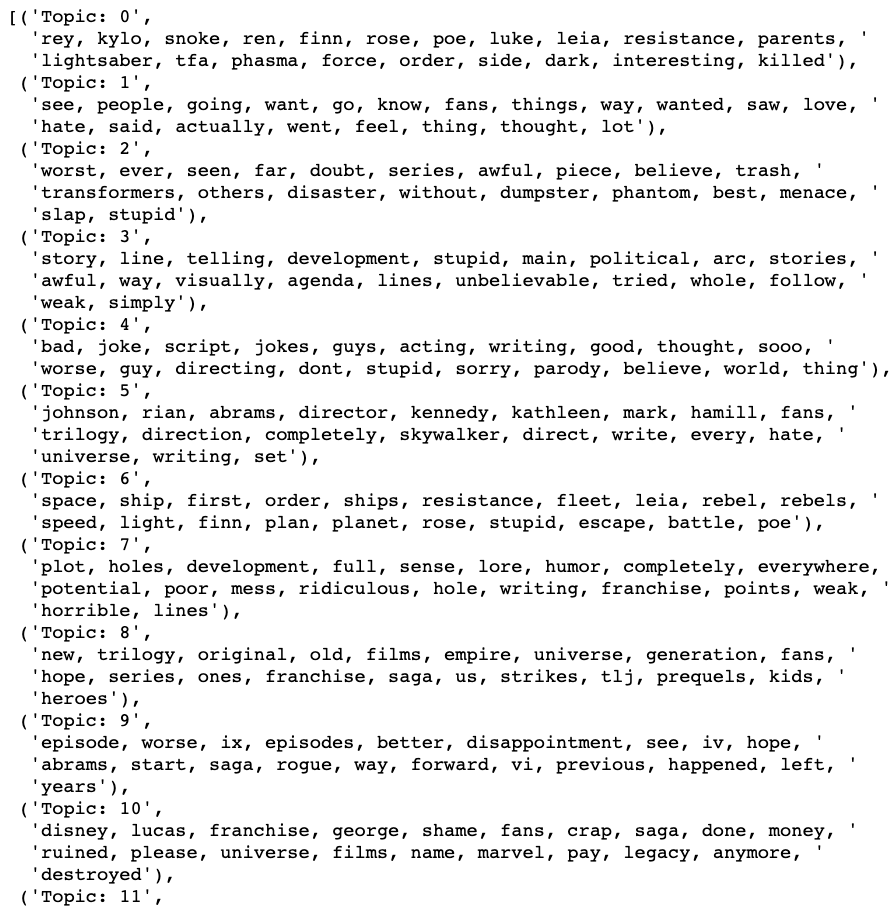
Topic 2 is raw, uncut negative sentiment, interestingly collecting together words that relate to garbage (“trash”, “dumpster”). Other deal with socio-political agendas, bad humor, the director, producers and Disney, indicating franchise stewardship, story and some plot-specific items. The main point though is that the topics were much clearer to see. Overall, NMF was producing much better results than LDA.

Another quite important observation is that, NMF executes much faster than LDA as well, roughly ~7-10x faster. At this point NMF is outperforming in all categories:

• LDA Exeuction Time (20 Topics): 20.07
• NMF Execution Time (20 Topics): 2.80

Next thing was to try higher n-gram processing, bigrams and trigrams.

Bigrams and Trigrams

Because 20 topics produced the best results for 1-grams I stuck with that topic number for bigrams and trigrams.

Bigrams generated topics aren’t that different from the non-bigram model, but there is a bit more clarity on some topics and one genuinely new one about the film being an “assembly line” creation, seen in Topic 12.

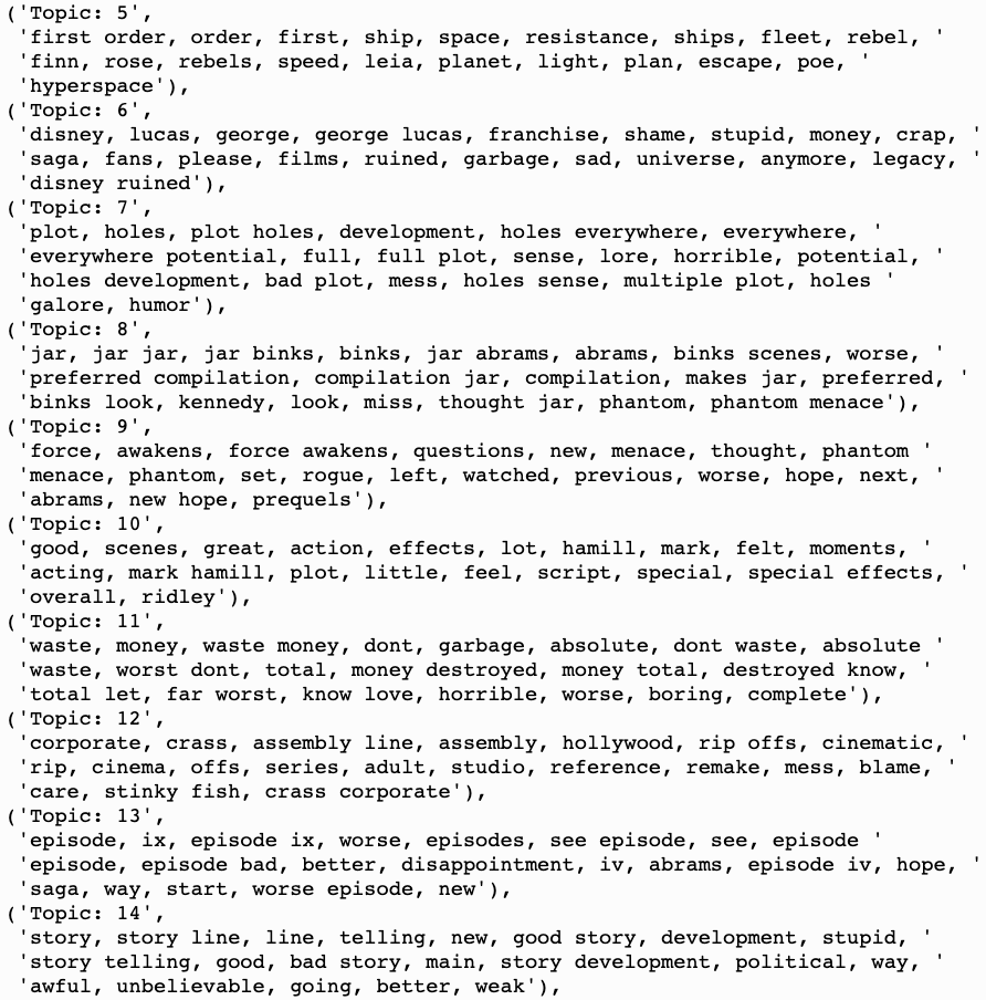
Overall I like the bigrams output slightly better, but it’s worth noting that the execution time is much longer, almost 30x longer.

• 1-grams Execution Time: 2.80
• Bigrams Execution Time: 57.72

If performance is a significant consideration I would go with the 1-grams model.

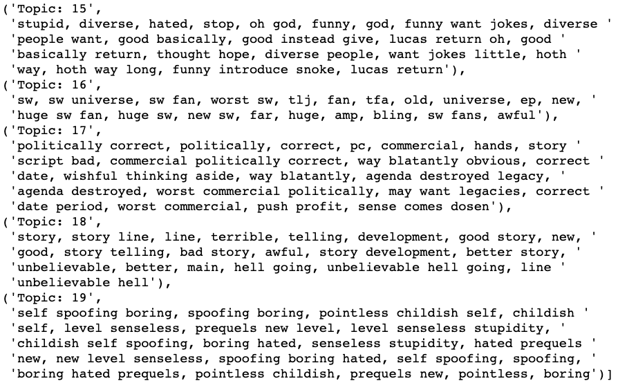
I next moved on to trigrams. The topic results for trigrams are similar to the bigrams results in several ways:

• Improved Results - Trigrams are a bit of an improvement over the 1-grams model, though not dramatically so.
• New Topics - Trigrams revealed a couple of unique subjects that weren’t present in both the default model and the bigrams model. It had the interesting “corporate assembly line production/stinky fish” topic and the “jar jar” comparisons topic. However it had these new topics as well:
  • Topic 15: Diversity as a specific problem
  • Topic 17: Political correctness
  • Topic 19: Childish “self-spoofing”

• Longer Execution Time - Trigrams also took much longer to run. It took ~3x as long as bigrams and ~75x times as long as the default model. Again, something to bear in mind.
  • 1-grams Execution Time: 2.80
  • Bigrams Execution Time: 57.72
  • Trigrams Execution Time: 146.75

If execution time was not an issue NMF trigrams would be the easy choice__. However, if execution time is a concern, and it often is, then you’ll have to make choices about what level of model effectiveness you want versus how long you’re willing to wait for them__. If this is in the middle of a live pipeline then it could become a significant bottleneck.

However, there may be ways to keep both model performance and execution time with additional optimization. This is definitely an area to explore.

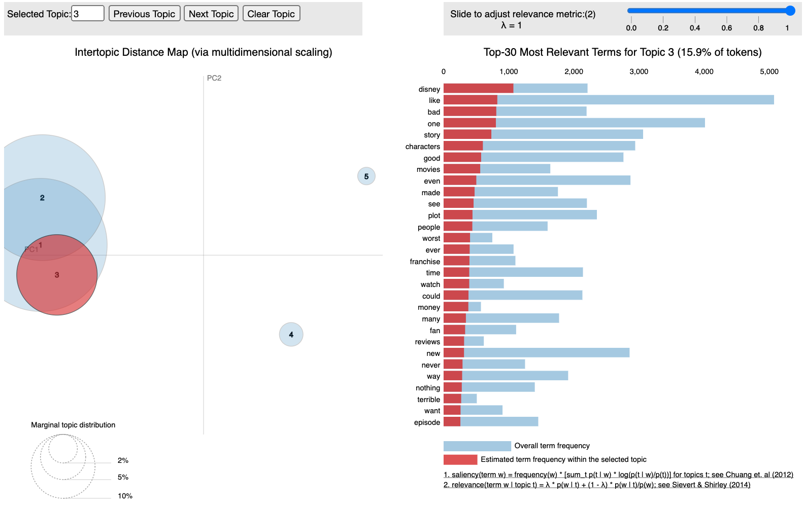
Finally, let’s look at the visualization in pyLDAvis, since the difference versus LDA is striking. Below is the visualization for trigrams in NMF, but the bigrams visualization is very similar:

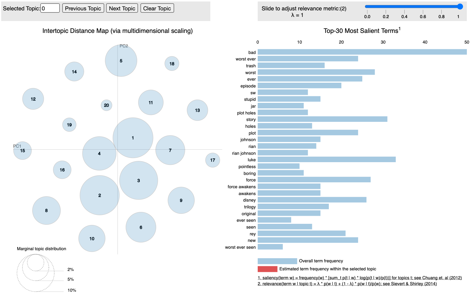
Notice how there is clean separation amongst all topics and that the term distribution amongst topics is more balanced. This is better than what we were seeing in LDA in just about every way, and it is good to note that the pyLDAvis plot seems to be a good indicator of whether or not you have decent topics, as the topics themselves are much better too.

All n-grams versions of NMF with 20 topics produced topics that were at least somewhat intelligible across all of the topics. Bigrams kept all of the topics from 1-grams and revealed even more and trigrams improved upon bigrams.

6. CONCLUSIONS

• In terms of sentiment analysis the Google Cloud Platform Natural Language API performed best. Even without any adjustments it outperformed the NLTK sentiment analysis in terms of getting closer to the actual sentiments of the reviews. However, the Google API generated many false positives for the negative category. Additional tweaking of the implementation may produce better results.
• Using LDA for topic modeling ultimately ended up not performing very well, at least for this project. It was relatively slow in terms of execution and the topic results were lackluster. At the very least it provided a baseline for comparison.
• NMF performed much better than LDA across the board. It was simpler to implement and the 1-grams implementation produced better topic results and was 10x faster than LDA.
• The best implementations of NMF were the bigrams and trigrams processed versions. All topics were somewhat intelligible and some were extremely clear and progressively revealed more interesting ideas.
• The one major catch was that NMF bigrams and trigrams were the slowest algorithms to run. If performance is a concern then 1-grams is probably the way to go, as it outperforms LDA in terms of topics and is 30-75x faster than bigrams and trigrams.
• So if performance is a concern, go with 1-grams NMF and if not go with bigrams or trigrams NMF.

7. Future Work

A lot of work was done between the sentiment analysis and topic modeling for this project and it produced some interesting and useful results, but I’m confident that more more work could be done to produce an even more useful model. Here are some future tasks that I think could effectively build upon it:

• Additional Reviews: The initial plan was actually to use 4 sources instead of 1. I would like to gather user reviews from Metacritic, Rotten Tomatoes and Amazon reviews of the blu-ray disc and digital versions of the film. With this I would have a bigger dataset to work with and also to have a wider variety of sources, perhaps yielding different ideas and insights. This could increase the clarity of the topics and accuracy of the approach.
• Twitter/Reddit: Getting impressions from Twitter and Reddit would be useful too, as we can capture both very short form and longer form impressions of the film. These are both very popular forums for opinion and the models would benefit from their inclusion.
• Different Movies/Games: I would also like to see how applicable the overall approach is to other films as well as games. Proving that this approach is generalizable would increase its value.
• Application: I think one of the most useful incarnations of these models is in application/dashboard form where the dashboard would show the trending topics for a film/game, various stats on those topics and allow you to drill down onto a specific topic and serve up tweets, Reddit posts and reviews that are related to it. Topics are interesting and useful, but ultimately content-creators will want to see opinions in detail. Long term perhaps there could be a service that will actually effectively summarize sentiment to the point where needing to read individual posts in detail will not be necessary, but I think content creators still want to see full posts and to better understand the context and get as close as possible to the opinion a person is actually expressing.

8. Resources

• GitHub Repository - GitHub repository containing all code, notebooks and data.

• Presentation Deck - This is a PowerPoint presentation deck created for a live presentation of project results.